DATASCI 350 - Data Science Computing

Lecture 22 - SQL Revision with DuckDB

Danilo Freire

danilo.freire@emory.edu

Department of Data and Decision Sciences
Emory University

Hello again! 😊

Brief recap 📚

Parallel computing fundamentals

Where lecture 21 left us

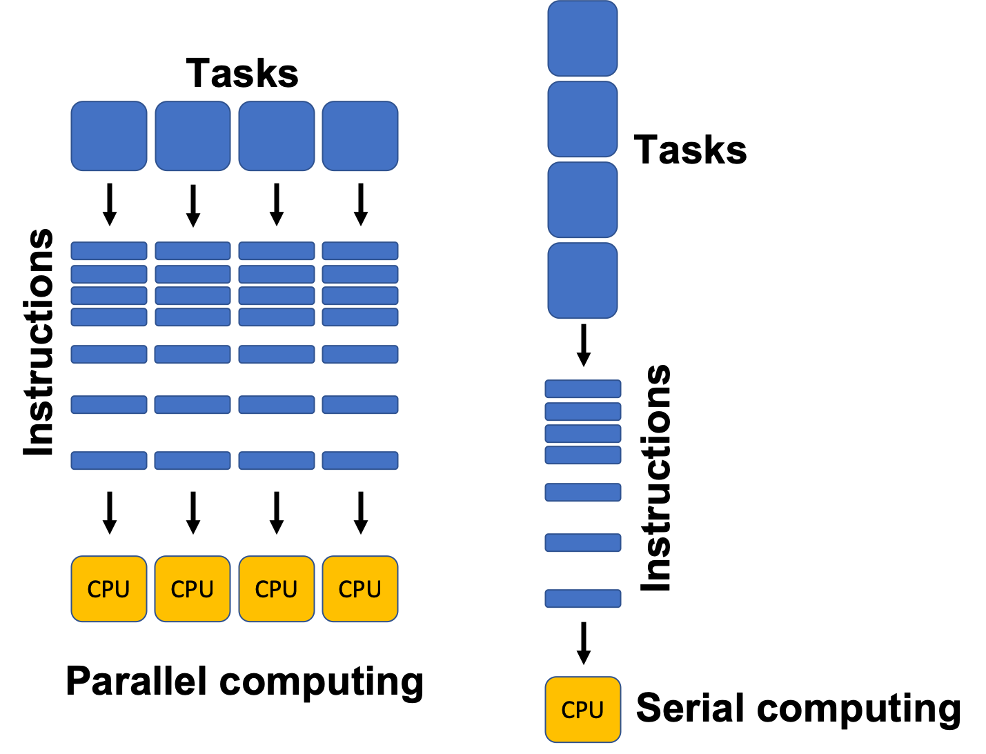
• Last class: parallel and scalable computing
  • map, joblib and concurrent.futures
  • Big O: parallelism divides the time, but not the growth rate
  • Amdahl’s law: the serial share limits the speed-up
  • The GIL: threads for waiting, processes for computing
  • Dask: lazy arrays and DataFrames for data bigger than RAM

• Some engines use all your cores with no setup
• DuckDB is one of them, and today we use it to revise SQL
• All queries run on the WDI panel from Lecture 19
• Download it here or use the path ../lecture-19/data/wdi_panel.parquet

Lecture overview

What we will cover today

1. Why SQL and why DuckDB

• A declarative language every engine speaks
• import duckdb is the whole setup

2. First queries

• SELECT, WHERE, ORDER BY, LIMIT
• IN, BETWEEN, LIKE, and the order a query runs in

3. Aggregating

• COUNT, AVG, GROUP BY, HAVING
• What COUNT does when values are missing

4. NULLs, CASE and windows

• IS NULL, COALESCE, income bands with CASE
• Window functions: a group mean and a rank on every row

5. Joins

• Primary keys, foreign keys, and the ON clause
• INNER, LEFT, FULL OUTER on two tiny tables

6. DuckDB and pandas

• Querying a pandas DataFrame by its variable name
• Handing a result back with .df()
• DuckDB on 200 million rows

Why SQL, why DuckDB 🦆

Why SQL

You describe the answer, the engine finds it

• SQL is a language for asking questions of tables
• It is relational: tables of rows and columns, combined with joins
• It is declarative: you say what you want, and the engine decides how
  • No loops, no variables, no input/output code
  • The engine can reorder the query, skip columns, or use every core
• SQL is about fifty years old, and tech job adverts list it about as often as Python
• SELECT, WHERE, GROUP BY and JOIN work the same in DuckDB, SQLite, PostgreSQL, BigQuery and Snowflake

DuckDB’s SQL introduction: https://duckdb.org/docs/stable/sql/introduction

Why DuckDB for a revision class

An in-process engine with no setup

• Zero setup: pip install duckdb, then import duckdb
• Unlike PostgreSQL, there is no server, user or password
• In-process: it runs inside your Python session, like SQLite
• Reads files by name: a Parquet or CSV path goes straight in FROM
• It reads a pandas DataFrame by its variable name too
• Columnar and parallel, so the same GROUP BY works on 200 million rows
• Version used here: DuckDB 1.5.5

Source: https://duckdb.org

First queries

What a table is

Rows, columns and one value per cell

• A table is a grid: each row is an observation, each column a variable
• Each column has one type. Ours are text (VARCHAR), whole numbers (SMALLINT) and decimals (DOUBLE)
• Other common types: BOOLEAN (true or false), DATE and TIMESTAMP
• A cell holds one value, or nothing: NULL
• The WDI panel: 217 countries, 8 indicators, 34 years (1990 to 2023)
• The number is always in value. The indicator column says what it measures
• So most queries start with WHERE indicator = '...', or they mix dollars with years of life
• In pandas terms: a table is a DataFrame, a column is a Series, and there is no index

Six rows of the panel, for Brazil in 2019 and 2020:

country	iso3	indicator	year	value
Brazil	BRA	gdp_per_capita	2019	8771.44
Brazil	BRA	gdp_per_capita	2020	8435.01
Brazil	BRA	internet_users_pct	2019	73.91
Brazil	BRA	internet_users_pct	2020	81.34
Brazil	BRA	life_expectancy	2019	75.81
Brazil	BRA	life_expectancy	2020	74.51

No two rows share the same country, indicator and year. Together they identify a row: the idea behind a primary key

Querying a Parquet file

The file path goes in the FROM clause

• The WDI panel is a Parquet file with 59,024 rows
• Download it here or use the path ../lecture-19/data/wdi_panel.parquet
• duckdb.sql() takes a query string and returns a result you can print
• The path goes in single quotes: single quotes mean text, double quotes a column name
• No read_parquet, connection or fetchall() needed. DuckDB handles it
• The column types under the names come from the file

import duckdb

duckdb.sql("""
    SELECT *
    FROM '../lecture-19/data/wdi_panel.parquet'
    LIMIT 5
""")

┌─────────┬─────────┬────────────────┬───────┬──────────────────┐
│ country │  iso3   │   indicator    │ year  │      value       │
│ varchar │ varchar │    varchar     │ int16 │      double      │
├─────────┼─────────┼────────────────┼───────┼──────────────────┤
│ Aruba   │ ABW     │ co2_per_capita │  1990 │ 3.20303411789078 │
│ Aruba   │ ABW     │ co2_per_capita │  1991 │ 3.43571688721622 │
│ Aruba   │ ABW     │ co2_per_capita │  1992 │  3.6345192377364 │
│ Aruba   │ ABW     │ co2_per_capita │  1993 │ 3.41453484426953 │
│ Aruba   │ ABW     │ co2_per_capita │  1994 │ 3.68322701204975 │
└─────────┴─────────┴────────────────┴───────┴──────────────────┘

Creating a view

One name for the file

• A view is a saved query that behaves like a table
• CREATE OR REPLACE VIEW wdi AS ... names the query wdi
• Later queries say FROM wdi, with no file path
• A view holds no data: DuckDB re-reads the file each time
• OR REPLACE overwrites an old view, so the cell is safe to re-run
• COUNT(DISTINCT country) counts the different values in a column
• The view disappears when Python restarts

duckdb.sql("""
    CREATE OR REPLACE VIEW wdi AS
    SELECT * FROM '../lecture-19/data/wdi_panel.parquet'
""")

duckdb.sql("""
    SELECT COUNT(*) AS n_rows,
           COUNT(DISTINCT country) AS countries,
           COUNT(DISTINCT indicator) AS indicators
    FROM wdi
""")

┌────────┬───────────┬────────────┐
│ n_rows │ countries │ indicators │
│ int64  │   int64   │   int64    │
├────────┼───────────┼────────────┤
│  59024 │       217 │          8 │
└────────┴───────────┴────────────┘

DESCRIBE and SUMMARIZE

Two commands to run before any query

• Run both before writing a query, to learn the column names
• DESCRIBE lists the columns and their types
• country, iso3 and indicator are text (VARCHAR), so filters on them need single quotes
• SUMMARIZE adds min, max, count and the share of missing values
• 11.06% of value is missing. country and year have no gaps
• Its result is a table, so we can SELECT from it
• In pandas: df.dtypes and df.describe()

duckdb.sql("DESCRIBE SELECT * FROM wdi")

┌─────────────┬─────────────┬─────────┬─────────┬─────────┬─────────┐
│ column_name │ column_type │  null   │   key   │ default │  extra  │
│   varchar   │   varchar   │ varchar │ varchar │ varchar │ varchar │
├─────────────┼─────────────┼─────────┼─────────┼─────────┼─────────┤
│ country     │ VARCHAR     │ YES     │ NULL    │ NULL    │ NULL    │
│ iso3        │ VARCHAR     │ YES     │ NULL    │ NULL    │ NULL    │
│ indicator   │ VARCHAR     │ YES     │ NULL    │ NULL    │ NULL    │
│ year        │ SMALLINT    │ YES     │ NULL    │ NULL    │ NULL    │
│ value       │ DOUBLE      │ YES     │ NULL    │ NULL    │ NULL    │
└─────────────┴─────────────┴─────────┴─────────┴─────────┴─────────┘

duckdb.sql("""
    SELECT column_name, min, max, null_percentage
    FROM (SUMMARIZE SELECT country, year, value FROM wdi)
""")

┌─────────────┬─────────────┬──────────────┬─────────────────┐
│ column_name │     min     │     max      │ null_percentage │
│   varchar   │   varchar   │   varchar    │  decimal(9,2)   │
├─────────────┼─────────────┼──────────────┼─────────────────┤
│ country     │ Afghanistan │ Zimbabwe     │            0.00 │
│ year        │ 1990        │ 2023         │            0.00 │
│ value       │ 0.0         │ 1438069596.0 │           11.06 │
└─────────────┴─────────────┴──────────────┴─────────────────┘

SELECT, aliases, ORDER BY, LIMIT

Picking columns and sorting the result

• The query is a Python string passed to duckdb.sql()
• Keywords are upper case by convention, but select works too, and Country finds country
• SELECT lists the columns you want. * means all of them
• It can compute new columns, like ROUND(value, 0)
• AS gives a column a new name, called an alias
• ORDER BY value DESC sorts high to low. ASC, low to high, is the default
• LIMIT keeps the first rows, like .head() in pandas

duckdb.sql("""
    SELECT country, year,
           ROUND(value, 0) AS gdp_pc
    FROM wdi
    WHERE indicator = 'gdp_per_capita'
      AND year = 2020
    ORDER BY value DESC
    LIMIT 5
""")

┌─────────────┬───────┬──────────┐
│   country   │ year  │  gdp_pc  │
│   varchar   │ int16 │  double  │
├─────────────┼───────┼──────────┤
│ Monaco      │  2020 │ 161263.0 │
│ Luxembourg  │  2020 │ 105274.0 │
│ Bermuda     │  2020 │  98846.0 │
│ Isle of Man │  2020 │  86595.0 │
│ Switzerland │  2020 │  86294.0 │
└─────────────┴───────┴──────────┘

WHERE with AND, OR and NOT

Filtering rows with WHERE

• WHERE keeps rows where the condition is true, like boolean indexing in pandas
• Comparisons: =, <> (not equal), <, <=, >, >=
• AND needs both sides true. OR needs either
• NOT flips a condition: NOT country = 'Japan' would keep only Brazil
• Text goes in single quotes, and the match is case-sensitive
• The brackets matter, because AND is applied before OR
• Four rows: Brazil on 6,818 and 8,435, Japan on 31,779 and 35,363

duckdb.sql("""
    SELECT country, year,
           ROUND(value, 0) AS gdp_pc
    FROM wdi
    WHERE indicator = 'gdp_per_capita'
      AND (year = 2000 OR year = 2020)
      AND (country = 'Brazil' OR country = 'Japan')
    ORDER BY country, year
""")

┌─────────┬───────┬─────────┐
│ country │ year  │ gdp_pc  │
│ varchar │ int16 │ double  │
├─────────┼───────┼─────────┤
│ Brazil  │  2000 │  6818.0 │
│ Brazil  │  2020 │  8435.0 │
│ Japan   │  2000 │ 31779.0 │
│ Japan   │  2020 │ 35363.0 │
└─────────┴───────┴─────────┘

Without the brackets, the query returns 496 rows: GDP for every country in 2000, all of Brazil’s 2020 rows, and every Japanese row

IN and BETWEEN

Shorter ways to write the same conditions

• IN replaces a chain of ORs on one column
• country IN ('Brazil', 'China') means country = 'Brazil' OR country = 'China'
• BETWEEN includes both ends: 2018 to 2020 covers three years
• The low end goes first. BETWEEN 2020 AND 2018 returns nothing
• In pandas: .isin([...]) and .between(2018, 2020)
• Six countries × three years = 18 rows. LIMIT 6 shows Brazil and China

duckdb.sql("""
    SELECT country, year,
           ROUND(value, 0) AS gdp_pc
    FROM wdi
    WHERE indicator = 'gdp_per_capita'
      AND country IN ('Brazil', 'China', 'Germany',
                      'India', 'Japan', 'United States')
      AND year BETWEEN 2018 AND 2020
    ORDER BY country, year
    LIMIT 6
""")

┌─────────┬───────┬─────────┐
│ country │ year  │ gdp_pc  │
│ varchar │ int16 │ double  │
├─────────┼───────┼─────────┤
│ Brazil  │  2018 │  8722.0 │
│ Brazil  │  2019 │  8771.0 │
│ Brazil  │  2020 │  8435.0 │
│ China   │  2018 │  9799.0 │
│ China   │  2019 │ 10356.0 │
│ China   │  2020 │ 10573.0 │
└─────────┴───────┴─────────┘

LIKE and ILIKE

Matching part of a text value

• LIKE matches part of a text value
• % means any characters, or none. _ means exactly one character
• 'United%' starts with United, '%States' ends with States, '%King%' contains King
• DISTINCT removes duplicates. Without it, each country appears once per indicator and year
• LIKE is case-sensitive, so 'united%' finds nothing
• ILIKE ignores case, and finds the same three countries
• In pandas: .str.startswith() or .str.contains()

duckdb.sql("""
    SELECT DISTINCT country
    FROM wdi
    WHERE country LIKE 'United%'
    ORDER BY country
""")

┌──────────────────────┐
│       country        │
│       varchar        │
├──────────────────────┤
│ United Arab Emirates │
│ United Kingdom       │
│ United States        │
└──────────────────────┘

duckdb.sql("""
    SELECT DISTINCT country
    FROM wdi
    WHERE country ILIKE 'united%'
    ORDER BY country
""")

┌──────────────────────┐
│       country        │
│       varchar        │
├──────────────────────┤
│ United Arab Emirates │
│ United Kingdom       │
│ United States        │
└──────────────────────┘

One query, one clause at a time

Every clause you have met, in one query

Clause	What it does
FROM wdi	picks the table
WHERE	keeps 6 of 59,024 rows
SELECT	picks 3 columns, rounds one
ORDER BY	sorts by value
LIMIT	keeps 3 rows

• You have met every clause here
• Read a query from FROM, because that is where the engine starts
• Three rows survive: the United States (59,534), Germany (42,373) and Japan (35,363)
• We build on this query for the rest of the lecture

duckdb.sql("""
    SELECT country, year, ROUND(value, 0) AS gdp_pc
    FROM wdi
    WHERE indicator = 'gdp_per_capita'
      AND country IN ('Brazil', 'China', 'Germany',
                      'India', 'Japan', 'United States')
      AND year = 2020
    ORDER BY value DESC
    LIMIT 3
""")

┌───────────────┬───────┬─────────┐
│    country    │ year  │ gdp_pc  │
│    varchar    │ int16 │ double  │
├───────────────┼───────┼─────────┤
│ United States │  2020 │ 59534.0 │
│ Germany       │  2020 │ 42373.0 │
│ Japan         │  2020 │ 35363.0 │
└───────────────┴───────┴─────────┘

The order a query really runs in

How the engine evaluates a query

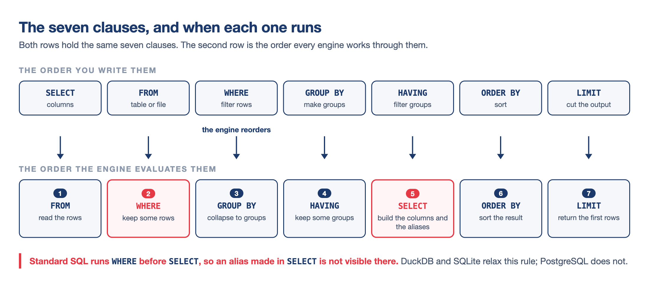
• You write SELECT first, but the engine runs it fifth
• FROM finds the rows, WHERE filters them, GROUP BY makes groups, HAVING filters groups, then SELECT builds the output
• ORDER BY sorts what SELECT produced, and LIMIT runs last of all

• An aggregate cannot go in WHERE: the groups do not exist yet
• Standard SQL rejects a SELECT alias in WHERE, because the alias does not exist yet. DuckDB allows it
• pandas writes the steps in this order: df[mask].groupby(...).agg(...)

Aggregating

GROUP BY

One row of output per group

• An aggregate function turns many rows into one number
• The common ones: COUNT, SUM, AVG (mean), MIN, MAX
• Without GROUP BY, the whole table is one group, so you get one row
• GROUP BY country makes six groups, so six rows
• Every column in SELECT must be in GROUP BY or inside an aggregate
  • SELECT country, value ... GROUP BY country fails: each group has 14 values, and SQL will not pick one
• n is 14: the years 2010 to 2023. In pandas: .groupby("country").agg(...)
• Two grouping columns give one row per pair: Appendix 04

duckdb.sql("""
    SELECT country,
           COUNT(value) AS n,
           ROUND(AVG(value), 0) AS mean_gdp
    FROM wdi
    WHERE indicator = 'gdp_per_capita'
      AND country IN ('Brazil', 'China', 'Germany',
                      'India', 'Japan', 'United States')
      AND year >= 2010
    GROUP BY country
    ORDER BY mean_gdp DESC
""")

┌───────────────┬───────┬──────────┐
│    country    │   n   │ mean_gdp │
│    varchar    │ int64 │  double  │
├───────────────┼───────┼──────────┤
│ United States │    14 │  58330.0 │
│ Germany       │    14 │  42448.0 │
│ Japan         │    14 │  35682.0 │
│ China         │    14 │   9017.0 │
│ Brazil        │    14 │   8923.0 │
│ India         │    14 │   1694.0 │
└───────────────┴───────┴──────────┘

WHERE and HAVING

Filtering before and after grouping

• WHERE filters rows before grouping. HAVING filters groups after
• Only HAVING can use an aggregate, because the groups exist by then
• “Which years count?” is about rows, so it goes in WHERE
• “Which countries qualify?” is about groups, so it goes in HAVING
• HAVING AVG(value) > 30000 keeps three countries
• China (9,017), Brazil (8,923) and India (1,694) drop out
• ORDER BY can use the alias mean_gdp, because it runs after SELECT

duckdb.sql("""
    SELECT country,
           COUNT(value) AS n,
           ROUND(AVG(value), 0) AS mean_gdp
    FROM wdi
    WHERE indicator = 'gdp_per_capita'
      AND country IN ('Brazil', 'China', 'Germany',
                      'India', 'Japan', 'United States')
      AND year >= 2010
    GROUP BY country
    HAVING AVG(value) > 30000
    ORDER BY mean_gdp DESC
""")

┌───────────────┬───────┬──────────┐
│    country    │   n   │ mean_gdp │
│    varchar    │ int64 │  double  │
├───────────────┼───────┼──────────┤
│ United States │    14 │  58330.0 │
│ Germany       │    14 │  42448.0 │
│ Japan         │    14 │  35682.0 │
└───────────────┴───────┴──────────┘

COUNT(*) and COUNT(value)

Counting rows and counting values

• COUNT(*) counts rows
• COUNT(value) counts only the rows where value is present
• The difference is the number of missing values
• AVG, SUM, MIN and MAX skip missing values without warning
• 217 countries a year: 25 missing in 1990, 18 in 2000, 9 in 2020
• So GDP coverage improves over time
• In pandas: len(df) against df["value"].count()
• Check this before you trust a mean

duckdb.sql("""
    SELECT year,
           COUNT(*) AS n_rows,
           COUNT(value) AS with_value,
           COUNT(*) - COUNT(value) AS missing
    FROM wdi
    WHERE indicator = 'gdp_per_capita'
      AND year IN (1990, 2000, 2020)
    GROUP BY year
    ORDER BY year
""")

┌───────┬────────┬────────────┬─────────┐
│ year  │ n_rows │ with_value │ missing │
│ int16 │ int64  │   int64    │  int64  │
├───────┼────────┼────────────┼─────────┤
│  1990 │    217 │        192 │      25 │
│  2000 │    217 │        199 │      18 │
│  2020 │    217 │        208 │       9 │
└───────┴────────┴────────────┴─────────┘

NULLs, CASE and windows

Missing values

Working with NULL

• NULL means “unknown”. It is not zero, and not an empty string
• Any comparison with NULL gives NULL, so NULL = NULL never matches
• Test with IS NULL or IS NOT NULL
• COALESCE(a, b) returns a, or b if a is NULL
• Yemen has no 2020 GDP figure, so it shows 0 here
• Filling with 0 is a choice. A mean over this column would be wrong
• COALESCE fills a missing value. A missing row needs a LEFT JOIN
• In pandas, NULL is NaN, and .fillna(0) does this

duckdb.sql("""
    SELECT country,
           ROUND(COALESCE(value, 0), 0) AS gdp_filled
    FROM wdi
    WHERE indicator = 'gdp_per_capita' AND year = 2020
      AND country IN ('Brazil', 'China', 'Germany', 'India',
                      'Japan', 'United States', 'Yemen, Rep.')
    ORDER BY country
""")

┌───────────────┬────────────┐
│    country    │ gdp_filled │
│    varchar    │   double   │
├───────────────┼────────────┤
│ Brazil        │     8435.0 │
│ China         │    10573.0 │
│ Germany       │    42373.0 │
│ India         │     1807.0 │
│ Japan         │    35363.0 │
│ United States │    59534.0 │
│ Yemen, Rep.   │        0.0 │
└───────────────┴────────────┘

CASE

Writing an if-else ladder inside a SELECT

• CASE is an if-else ladder inside SELECT
• WHEN gives a condition, and THEN the value to use if it holds
• Tests run top to bottom, and the first true one wins
• ELSE catches the rest, and END closes the ladder. Without ELSE, unmatched rows get NULL
• The cut-offs are the World Bank’s FY24 income bands. The Bank applies them to GNI per capita, so here they are a rough guide
• IS NULL comes first on purpose. Lower down, Yemen would fall to ELSE as “Low income”
• The result is a new column you can group, join, or export

duckdb.sql("""
    SELECT country, ROUND(value, 0) AS gdp_pc,
        CASE
            WHEN value IS NULL  THEN 'No data'
            WHEN value >= 13846 THEN 'High income'
            WHEN value >= 4466  THEN 'Upper middle'
            WHEN value >= 1136  THEN 'Lower middle'
            ELSE 'Low income'
        END AS income_band
    FROM wdi
    WHERE indicator = 'gdp_per_capita' AND year = 2020
      AND country IN ('Brazil', 'China', 'Germany', 'India',
                      'Japan', 'United States', 'Yemen, Rep.')
    ORDER BY value DESC NULLS LAST
""")

┌───────────────┬─────────┬──────────────┐
│    country    │ gdp_pc  │ income_band  │
│    varchar    │ double  │   varchar    │
├───────────────┼─────────┼──────────────┤
│ United States │ 59534.0 │ High income  │
│ Germany       │ 42373.0 │ High income  │
│ Japan         │ 35363.0 │ High income  │
│ China         │ 10573.0 │ Upper middle │
│ Brazil        │  8435.0 │ Upper middle │
│ India         │  1807.0 │ Lower middle │
│ Yemen, Rep.   │    NULL │ No data      │
└───────────────┴─────────┴──────────────┘

Window functions

A group-level number on every row

• GROUP BY year would collapse these 12 rows into 2
• A window function keeps every row and adds a group number beside it
• OVER turns an aggregate into a window function
• PARTITION BY year makes one window, a set of rows, per year. No rows are lost
• year_mean repeats on each row of its year: 20,885 in 2000, 26,347 in 2020
• In pandas: .groupby("year")["value"].transform("mean")

duckdb.sql("""
    SELECT country, year, ROUND(value, 0) AS gdp_pc,
           ROUND(AVG(value) OVER (PARTITION BY year), 0)
               AS year_mean
    FROM wdi
    WHERE indicator = 'gdp_per_capita'
      AND country IN ('Brazil', 'China', 'Germany',
                      'India', 'Japan', 'United States')
      AND year IN (2000, 2020)
    ORDER BY year, value DESC
""")

┌───────────────┬───────┬─────────┬───────────┐
│    country    │ year  │ gdp_pc  │ year_mean │
│    varchar    │ int16 │ double  │  double   │
├───────────────┼───────┼─────────┼───────────┤
│ United States │  2000 │ 48616.0 │   20885.0 │
│ Germany       │  2000 │ 35104.0 │   20885.0 │
│ Japan         │  2000 │ 31779.0 │   20885.0 │
│ Brazil        │  2000 │  6818.0 │   20885.0 │
│ China         │  2000 │  2237.0 │   20885.0 │
│ India         │  2000 │   757.0 │   20885.0 │
│ United States │  2020 │ 59534.0 │   26347.0 │
│ Germany       │  2020 │ 42373.0 │   26347.0 │
│ Japan         │  2020 │ 35363.0 │   26347.0 │
│ China         │  2020 │ 10573.0 │   26347.0 │
│ Brazil        │  2020 │  8435.0 │   26347.0 │
│ India         │  2020 │  1807.0 │   26347.0 │
└───────────────┴───────┴─────────┴───────────┘
  12 rows                           4 columns

Ranking with a window

RANK() needs an ORDER BY inside OVER

• RANK() numbers rows by the ORDER BY inside OVER
• The inner ORDER BY sets the ranks. The outer one sorts the printed table
• No PARTITION BY: one window for the whole result
• Ties share a rank, and the next is skipped: 1, 2, 2, 4
• DENSE_RANK() gives 1, 2, 2, 3, and ROW_NUMBER() never ties
• The United States ranks 1 (59,534), and India 6 (1,807)
• WHERE runs first, so only these six countries are ranked
• Add PARTITION BY year to rank within each year

duckdb.sql("""
    SELECT country, ROUND(value, 0) AS gdp_pc,
           RANK() OVER (ORDER BY value DESC) AS rank_2020
    FROM wdi
    WHERE indicator = 'gdp_per_capita'
      AND country IN ('Brazil', 'China', 'Germany',
                      'India', 'Japan', 'United States')
      AND year = 2020
    ORDER BY rank_2020
""")

┌───────────────┬─────────┬───────────┐
│    country    │ gdp_pc  │ rank_2020 │
│    varchar    │ double  │   int64   │
├───────────────┼─────────┼───────────┤
│ United States │ 59534.0 │         1 │
│ Germany       │ 42373.0 │         2 │
│ Japan         │ 35363.0 │         3 │
│ China         │ 10573.0 │         4 │
│ Brazil        │  8435.0 │         5 │
│ India         │  1807.0 │         6 │
└───────────────┴─────────┴───────────┘

Joins

Two small tables

Keys, and the two tables we will join

• A table stores its data, unlike the wdi view
• CREATE TABLE ... AS SELECT builds gdp2020 from a query
• CREATE TABLE (col TYPE, ...) declares empty columns. INSERT INTO ... VALUES adds rows
• A primary key identifies each row, with no duplicates or NULLs: iso3 in regions
• A foreign key points at another table’s primary key. iso3 in gdp2020 plays that role, but we never declare it, so JPN can sit there with no partner
• Six rows in gdp2020, seven in regions
• Mismatches: JPN has GDP but no region. KOR and AUS have a region but no GDP
• East Asia holds two codes, which matters in the exercise

duckdb.sql("""
    CREATE OR REPLACE TABLE gdp2020 AS
    SELECT country, iso3, ROUND(value, 0) AS gdp_per_capita
    FROM wdi
    WHERE indicator = 'gdp_per_capita' AND year = 2020
      AND iso3 IN ('USA','BRA','CHN','IND','DEU','JPN')
""")

duckdb.sql("""
    CREATE OR REPLACE TABLE regions
        (iso3 VARCHAR PRIMARY KEY, region VARCHAR)
""")

duckdb.sql("""
    INSERT INTO regions VALUES
        ('USA', 'North America'), ('BRA', 'Latin America'),
        ('CHN', 'East Asia'),     ('IND', 'South Asia'),
        ('DEU', 'Europe'),        ('KOR', 'East Asia'),
        ('AUS', 'Oceania')
""")

duckdb.sql("SELECT * FROM regions ORDER BY iso3")

┌─────────┬───────────────┐
│  iso3   │    region     │
│ varchar │    varchar    │
├─────────┼───────────────┤
│ AUS     │ Oceania       │
│ BRA     │ Latin America │
│ CHN     │ East Asia     │
│ DEU     │ Europe        │
│ IND     │ South Asia    │
│ KOR     │ East Asia     │
│ USA     │ North America │
└─────────┴───────────────┘

Reading a join

The ON clause and table aliases

• A JOIN combines two tables into one wider result
• ON says which columns must match: iso3 on both sides
• Each matching pair of rows becomes one output row
• AS g and AS r are table aliases: short names for the tables
• g.country means “country from gdp2020”. Prefix every column this way
• The join type goes before JOIN. INNER is the default
• In pandas: pd.merge(gdp2020, regions, on="iso3")
• The next three slides run this with three join types

SELECT g.country, r.region, g.gdp_per_capita
FROM gdp2020 AS g
INNER JOIN regions AS r ON g.iso3 = r.iso3
ORDER BY g.country

INNER JOIN

Only the rows that match on both sides

• An INNER JOIN keeps only the codes in both tables
• Six rows on the left, seven on the right, five out
• Japan drops out: JPN is not in regions
• Korea and Australia drop out too: they have no 2020 GDP row
• An inner join filters silently, with no warning about lost rows
• If your row count falls after a join, this is usually why
• In pandas: pd.merge(..., how="inner")

duckdb.sql("""
    SELECT g.country, r.region, g.gdp_per_capita
    FROM gdp2020 AS g
    INNER JOIN regions AS r ON g.iso3 = r.iso3
    ORDER BY g.country
""")

┌───────────────┬───────────────┬────────────────┐
│    country    │    region     │ gdp_per_capita │
│    varchar    │    varchar    │     double     │
├───────────────┼───────────────┼────────────────┤
│ Brazil        │ Latin America │         8435.0 │
│ China         │ East Asia     │        10573.0 │
│ Germany       │ Europe        │        42373.0 │
│ India         │ South Asia    │         1807.0 │
│ United States │ North America │        59534.0 │
└───────────────┴───────────────┴────────────────┘

LEFT JOIN

Keeping every row of the left table

• A LEFT JOIN keeps every row of the left table
• The left table is the one in FROM: gdp2020 here
• Six rows: Japan is back, with NULL for region
• That NULL means “no partner found”. Japan’s 35,363 is unchanged
• Korea and Australia are still missing: they exist only on the right
• Swap the tables and you get a different answer, as in the exercise
• The join you will use most: it adds labels without losing rows
• In pandas: pd.merge(..., how="left")

duckdb.sql("""
    SELECT g.country, r.region, g.gdp_per_capita
    FROM gdp2020 AS g
    LEFT JOIN regions AS r ON g.iso3 = r.iso3
    ORDER BY g.country
""")

┌───────────────┬───────────────┬────────────────┐
│    country    │    region     │ gdp_per_capita │
│    varchar    │    varchar    │     double     │
├───────────────┼───────────────┼────────────────┤
│ Brazil        │ Latin America │         8435.0 │
│ China         │ East Asia     │        10573.0 │
│ Germany       │ Europe        │        42373.0 │
│ India         │ South Asia    │         1807.0 │
│ Japan         │ NULL          │        35363.0 │
│ United States │ North America │        59534.0 │
└───────────────┴───────────────┴────────────────┘

FULL OUTER JOIN

Every row from both tables survives

• A FULL OUTER JOIN keeps every row from both tables, with NULLs where there is no partner
• Eight rows: five pairs, plus Japan, Korea and Australia
• Korea and Australia have a region, but NULL country and gdp_per_capita
• Japan has a country and 35,363, but NULL region columns
• On these tables: 5 rows from INNER, 6 from LEFT, 8 from FULL OUTER
• To choose a join, ask which table must survive whole, and what to do with rows that have no partner

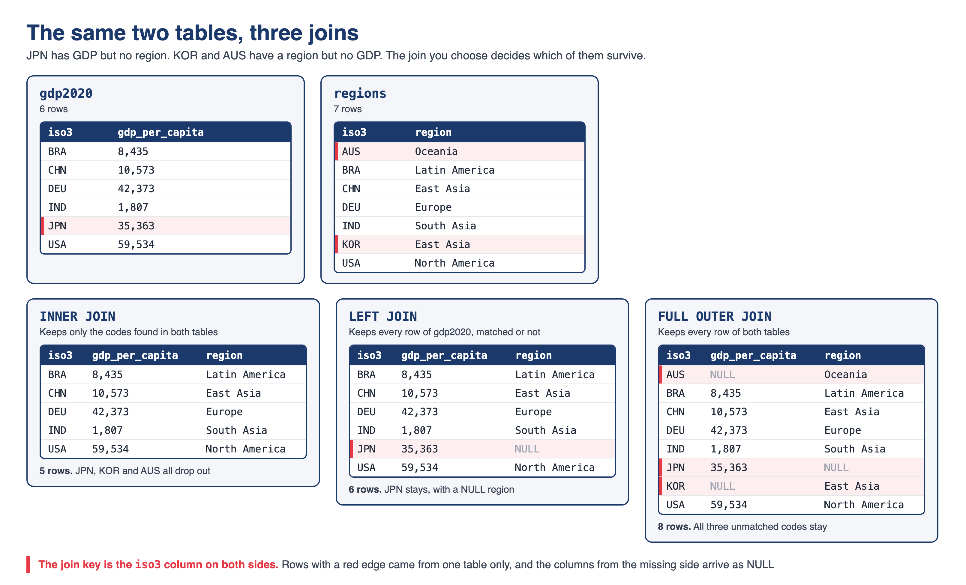
Our two tables and the three joins. Click to enlarge

duckdb.sql("""
    SELECT g.country, r.iso3 AS region_iso3,
           r.region, g.gdp_per_capita
    FROM gdp2020 AS g
    FULL OUTER JOIN regions AS r ON g.iso3 = r.iso3
    ORDER BY r.region NULLS LAST, r.iso3
""")

┌───────────────┬─────────────┬───────────────┬────────────────┐
│    country    │ region_iso3 │    region     │ gdp_per_capita │
│    varchar    │   varchar   │    varchar    │     double     │
├───────────────┼─────────────┼───────────────┼────────────────┤
│ China         │ CHN         │ East Asia     │        10573.0 │
│ NULL          │ KOR         │ East Asia     │           NULL │
│ Germany       │ DEU         │ Europe        │        42373.0 │
│ Brazil        │ BRA         │ Latin America │         8435.0 │
│ United States │ USA         │ North America │        59534.0 │
│ NULL          │ AUS         │ Oceania       │           NULL │
│ India         │ IND         │ South Asia    │         1807.0 │
│ Japan         │ NULL        │ NULL          │        35363.0 │
└───────────────┴─────────────┴───────────────┴────────────────┘

Try it yourself! 🧠

Ten minutes

How rich is each region, and how much data is it based on?

1. Use the gdp2020 and regions tables from the joins section
2. Report one row per region
3. Count how many of that region’s countries have a 2020 GDP figure
4. Compute the mean GDP per capita of that region
5. Keep every region, including the one with no GDP data at all
6. Sort by mean GDP, highest first
7. Send the region with no data to the bottom of the list

What to look for:

• Which table goes on the left if every region must survive?
• East Asia has two codes but one GDP figure, so COUNT(*) and COUNT(g.country) differ
• Oceania has no GDP figure at all
• Six regions come back

Solution: Appendix 01

DuckDB and pandas 🐼

Querying a DataFrame by name

Your Python variable becomes a SQL table

• DuckDB finds df among your Python variables and queries it by name
• No registration, no copy, no conversion: it reads the DataFrame in memory
• The same SELECT works on a file, a view or a DataFrame
• SELECT COUNT(*) FROM df gives 59,024, like the Parquet file
• You can join two DataFrames in one query

import pandas as pd

df = pd.read_parquet(
    "../lecture-19/data/wdi_panel.parquet"
)

duckdb.sql("SELECT COUNT(*) AS n FROM df")

┌───────┐
│   n   │
│ int64 │
├───────┤
│ 59024 │
└───────┘

country is a pandas category: a text column with a fixed list of allowed values. DuckDB calls this type an enum (short for enumeration). Add ::VARCHAR to turn it into plain text

Handing the result back to pandas

Turning a result into a DataFrame

• .df() turns a DuckDB result into a pandas DataFrame
• .pl() gives a Polars DataFrame, and .to_arrow_table() an Arrow table
• Without .df(), you get a DuckDB result that prints as a text table
• country::VARCHAR turns the category back into plain text
• SQL returns 18 rows, and pivot reshapes them into 6 rows by 3 columns
• DuckDB has a PIVOT statement too, but reshaping reads more easily in pandas
• After .df(), it is ordinary pandas: .plot(), .to_csv(), seaborn, statsmodels
• SQL or pandas? Appendix 06

long = duckdb.sql("""
    SELECT country::VARCHAR AS country, indicator,
           ROUND(value, 1) AS value
    FROM df
    WHERE year = 2020
      AND iso3 IN ('USA', 'BRA', 'CHN',
                   'IND', 'DEU', 'JPN')
      AND indicator IN ('gdp_per_capita',
                        'life_expectancy',
                        'internet_users_pct')
""").df()

long.pivot(index="country", columns="indicator",
           values="value")

indicator	gdp_per_capita	internet_users_pct	life_expectancy
country
Brazil	8435.0	81.3	74.5
China	10573.4	70.1	78.0
Germany	42372.9	89.8	81.0
India	1806.5	43.4	70.2
Japan	35363.3	90.2	84.6
United States	59533.6	90.3	77.0

DuckDB on 200 million rows

The same SQL on a 200-million-row file

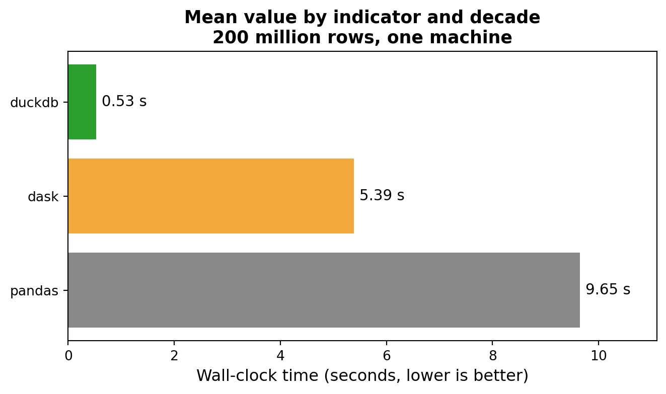
• Task: mean value by indicator and decade, on wdi_big.parquet, a synthetic panel of 200,681,600 rows
• DuckDB: 0.53 s. Dask: 5.39 s. pandas: 9.65 s
• pandas loads every column into RAM. DuckDB reads only the three columns the query uses
• Why: columnar storage, vectorised execution, and all cores by default
• MacBook Pro, Apple M5, 10 cores, 24 GB RAM, macOS 26.6
• Your seconds will differ, but the ranking usually holds
• Polars is in the same range as DuckDB (Tutorial 07)
• The query and scripts: Appendix 07

Summary

What we learned today

The vocabulary, in the order we met it

• SQL is declarative: you describe the answer and the engine plans the work
• DuckDB needs one import and reads a Parquet file or a pandas DataFrame by name
• A view names a query. DESCRIBE and SUMMARIZE show what is in it
• WHERE filters rows, GROUP BY forms groups, HAVING filters groups. No aggregate in WHERE
• COUNT(*) minus COUNT(value) is the number of missing values

• A NULL means unknown. COALESCE fills one in, and a missing row needs a join instead
• CASE builds a category column from an if-else ladder
• A window function keeps every row: AVG ... OVER (PARTITION BY year) adds the year mean, RANK() a position
• Joins: 5 rows from INNER, 6 from LEFT, 8 from FULL OUTER on the same two tables
• On 200 million rows, DuckDB runs the same query in 0.53 seconds

Next class

• Lecture 23: dependency management, virtual environments and containers
• Today’s queries depended on your Python, your DuckDB version and your laptop
• Next class we package all three into an image, so anyone who runs it gets the same answer
• pip install duckdb stops being a setup instruction and becomes a line in a Dockerfile

Before then:

1. Finish the join exercise if you did not complete it in class
2. Work through Tutorial 04, the DuckDB SQL tutorial on the course website
3. Check that import duckdb works in your environment
4. More practice with GROUP BY and HAVING: Appendix 02. Common error messages: Appendix 03

Thank you very much! 😊

Appendix 📚

Appendix 01: Solution to the exercise

• regions goes on the left, because every region must survive
• East Asia has two rows in regions, but COUNT(g.country) is 1: Korea’s row has a NULL country
• COUNT(*) would count that row and report 2
• Oceania has no GDP figure: its count is 0 and its mean is NULL
• NULLS LAST sends Oceania to the bottom
• Six regions, from North America (59,534) down to South Asia (1,807), then Oceania
• Codes that appear in only one table? Appendix 05

Back to the exercise

duckdb.sql("""
    SELECT r.region,
           COUNT(g.country) AS countries_with_gdp,
           ROUND(AVG(g.gdp_per_capita), 0) AS mean_gdp
    FROM regions AS r
    LEFT JOIN gdp2020 AS g ON g.iso3 = r.iso3
    GROUP BY r.region
    ORDER BY mean_gdp DESC NULLS LAST
""")

┌───────────────┬────────────────────┬──────────┐
│    region     │ countries_with_gdp │ mean_gdp │
│    varchar    │       int64        │  double  │
├───────────────┼────────────────────┼──────────┤
│ North America │                  1 │  59534.0 │
│ Europe        │                  1 │  42373.0 │
│ East Asia     │                  1 │  10573.0 │
│ Latin America │                  1 │   8435.0 │
│ South Asia    │                  1 │   1807.0 │
│ Oceania       │                  0 │     NULL │
└───────────────┴────────────────────┴──────────┘

Appendix 02: Practice at home: GROUP BY and HAVING

One more question to try on your own

Which countries have had the highest life expectancy since 2010?

1. Create the wdi view over the panel
2. Keep only the life_expectancy rows
3. Keep only the years from 2010 onwards
4. Compute the mean of value for each country
5. Keep the countries whose mean is above 82
6. Sort from highest to lowest
7. Return the top five, rounded to one decimal

duckdb.sql("""
    SELECT country,
           ROUND(AVG(value), 1) AS mean_life_exp
    FROM wdi
    WHERE indicator = 'life_expectancy'
      AND year >= 2010
    GROUP BY country
    HAVING AVG(value) > 82
    ORDER BY mean_life_exp DESC
    LIMIT 5
""")

┌──────────────────────┬───────────────┐
│       country        │ mean_life_exp │
│       varchar        │    double     │
├──────────────────────┼───────────────┤
│ Monaco               │          85.5 │
│ San Marino           │          84.4 │
│ Hong Kong SAR, China │          84.3 │
│ Japan                │          83.8 │
│ Andorra              │          83.8 │
└──────────────────────┴───────────────┘

• WHERE drops rows, HAVING AVG(value) > 82 tests the group
• ORDER BY names mean_life_exp, the alias created in SELECT
• Hong Kong and Japan are the only places in the top five with more than a million people

Back to Next class

Appendix 03: When something goes wrong

Parser Error: syntax error at or near ".."

The file path is not quoted. Put single quotes around it: FROM '../data/f.parquet'.

IO Error: No files found that match the pattern

The path is quoted but wrong. Paths are relative to the working directory (the notebook’s folder in Jupyter), so check with os.getcwd().

Binder Error: Referenced column "gdp" not found

The column name is misspelled or does not exist. Run DESCRIBE SELECT * FROM wdi and read the list

Parser Error: syntax error at or near "SELCT"

A keyword is misspelled. DuckDB quotes the offending word back at you, so read the message to the end.

Binder Error on a value you know exists

You wrote WHERE indicator = "gdp_per_capita" with double quotes. Double quotes mean a column name in SQL, single quotes mean text.

Catalog Error: Table with name wdi does not exist

The view lives in the session that created it. Re-run the CREATE VIEW cell after restarting Python

Back to Next class

Appendix 04: Grouping by two columns

Every combination that exists in the data

• Name two columns and you get one row for each pair that appears in the filtered rows
• Two countries and two indicators give four rows here
• Combinations with no rows never appear. SQL does not invent empty groups
• Japan’s mean life expectancy since 2010 is nine years above Brazil’s. Its CO2 per person is almost four times higher
• A mean over years like this weights every year equally. Say so when you report it

duckdb.sql("""
    SELECT country, indicator,
           ROUND(AVG(value), 1) AS mean_value
    FROM wdi
    WHERE year >= 2010
      AND country IN ('Brazil', 'Japan')
      AND indicator IN ('life_expectancy',
                        'co2_per_capita')
    GROUP BY country, indicator
    ORDER BY country, indicator
""")

┌─────────┬─────────────────┬────────────┐
│ country │    indicator    │ mean_value │
│ varchar │     varchar     │   double   │
├─────────┼─────────────────┼────────────┤
│ Brazil  │ co2_per_capita  │        2.4 │
│ Brazil  │ life_expectancy │       74.8 │
│ Japan   │ co2_per_capita  │        9.3 │
│ Japan   │ life_expectancy │       83.8 │
└─────────┴─────────────────┴────────────┘

Back to GROUP BY

Appendix 05: Anti-joins and UNION

Finding rows with no partner

• An anti-join asks which rows on the left have no partner on the right
• NOT EXISTS runs a small query for each row and keeps the row when it returns nothing
• Japan is the only such row here, because JPN is missing from regions
• A join adds columns. UNION stacks rows from two results that have the same columns
• UNION removes duplicate rows, UNION ALL keeps them and is faster
• The tagged result has five rows: Germany, Japan and the United States rich, Brazil and India poor
• China falls in neither band, so it appears in no row at all

duckdb.sql("""
    SELECT g.country, g.iso3
    FROM gdp2020 AS g
    WHERE NOT EXISTS (
        SELECT 1 FROM regions AS r
        WHERE r.iso3 = g.iso3
    )
""")

┌─────────┬─────────┐
│ country │  iso3   │
│ varchar │ varchar │
├─────────┼─────────┤
│ Japan   │ JPN     │
└─────────┴─────────┘

duckdb.sql("""
    SELECT country, 'rich' AS tag FROM gdp2020
    WHERE gdp_per_capita > 30000
    UNION
    SELECT country, 'poor' AS tag FROM gdp2020
    WHERE gdp_per_capita < 10000
    ORDER BY country
""")

┌───────────────┬─────────┐
│    country    │   tag   │
│    varchar    │ varchar │
├───────────────┼─────────┤
│ Brazil        │ poor    │
│ Germany       │ rich    │
│ India         │ poor    │
│ Japan         │ rich    │
│ United States │ rich    │
└───────────────┴─────────┘

Back to the exercise solution

Appendix 06: When SQL beats a DataFrame

A checklist for each tool

Reach for SQL when:

• You are joining two or more tables
• You are filtering and aggregating a file that is larger than your RAM
• The question is a GROUP BY with a couple of conditions
• Someone else has to read the query. A colleague who has never seen pandas can still read your SELECT
• The data already lives in a database

Stay in pandas when:

• You need row-by-row logic that has no set-based version
• You are plotting, or feeding a model
• You want many small inspectable steps, each one a variable you can look at
• The reshaping is the hard part, as in the pivot in the DuckDB and pandas section

Want more practice? The course website has a full self-study DuckDB SQL tutorial covering everything on these slides in more depth

Back to the pandas slide

Appendix 07: The benchmark query

The query and where the timings come from

• The DuckDB version is the query you already know, with a file path in FROM and a GROUP BY at the end
• The data is wdi_big.parquet, a synthetic panel of 200,681,600 rows built by cloning the small panel many times
• The file is not committed, and the script that rebuilds it is in data/make_big_parquet.py
• The timings were measured once and saved to data/benchmark_results.csv. The deck reads that file rather than re-running anything
• pandas loads the whole thing and calls groupby, Dask uses a parallel DataFrame, and DuckDB runs SQL straight over the file

import duckdb

duckdb.sql("""
    SELECT indicator,
           (year // 10) * 10 AS decade,
           AVG(value) AS mean_value
    FROM 'data/wdi_big.parquet'
    WHERE year >= 1990
    GROUP BY indicator, decade
""").df()

Back to the benchmark