DATASCI 350 - Data Science Computing

Lecture 21 - Parallel Computing Fundamentals

Danilo Freire

Department of Data and Decision Sciences
Emory University

Hello again, my friends! 😊

Brief recap 📚

Module 06: getting data from the web

What we did in lectures 18 and 19

  • A web API is a contract between your code and a server
  • We sent HTTP requests and read the JSON that came back
  • We handled pagination and wrapped the whole download in get_wdi()
  • Pages without an API need requests and BeautifulSoup instead
  • We saved every result as a parquet file, which keeps column types and compresses well
  • Today we ask what happens when those files get really big!
  • This module is called Scaling and Performance because “parallelise” is only one of the answers
  • Sometimes parallelism really is the right move
  • Sometimes the fix is a better algorithm
  • Sometimes we need a faster engine (next lecture)
  • We will cover all three strategies across these two lectures

Worth noticing: the parquet files we wrote in Module 06 are exactly the format Dask reads

Today’s agenda

Lecture outline

What we will cover today

  • Serial vs parallel execution
    • map function and embarrassingly parallel problems
  • Big O notation and what parallelism can (and cannot) fix
  • Amdahl’s law: the speed-up ceiling
  • The GIL: why threads do not always help in Python
  • joblib and concurrent.futures for single-node parallelism
  • Dask for scalable computing
    • Lazy evaluation: arrays and DataFrames
    • Reading and writing CSV and Parquet files
    • dask.delayed for custom pipelines
  • Best practices: when to parallelise and when not to

Serial vs parallel algorithms

Serial execution

One line finishes before the next one starts

  • A typical Python program runs its lines one after another, in order:
# Import packages
import numpy as np

# Define an array of numbers
foo = np.array([0, 1, 2, 3, 4, 5])

# Define a function that squares numbers
def bar(x):
    return x * x

# Loop over each element and perform an action on it
for element in foo:
    # Print the result of bar
    print(bar(element))
0
1
4
9
16
25

The map function

Apply one function to every element of a list

  • We will use a tool called map later in this lecture
  • It applies one function to each element of a list or array
  • Here is a version I wrote by hand so you can see the loop inside it:
# (Very) inefficient function
def my_map(function, array):
    # create a container for the results
    output = []

    # loop over each element
    for element in array:
        
        # add the intermediate result
        output.append(function(element))
    
    # return the now-filled container
    return output
my_map(bar, foo)
[np.int64(0),
 np.int64(1),
 np.int64(4),
 np.int64(9),
 np.int64(16),
 np.int64(25)]
list(map(bar, foo))
[np.int64(0),
 np.int64(1),
 np.int64(4),
 np.int64(9),
 np.int64(16),
 np.int64(25)]
  • The built-in version returns the same answer and runs much faster than mine (it is implemented in C), so use it instead

Using joblib for parallel computing

Two functions turn a loop into parallel work

  • Each step of our map call is independent, so nothing stops us running the steps at the same time
  • joblib gives us two functions for that
  • Parallel(n_jobs=k) runs k tasks at the same time
  • delayed(f) wraps f so that joblib can schedule the call instead of running it immediately
  • You combine them with a generator expression, as shown on the right
  • n_jobs=-1 asks joblib to use all available CPU cores
  • joblib handles process creation, data transfer and result collection for you
  • More details in the joblib documentation
  • Using our bar function and foo array from before:
# Install joblib if you haven't done so yet
# !pip install joblib

# Import joblib functions 
from joblib import Parallel, delayed

results = Parallel(n_jobs=6)(
    delayed(bar)(x) for x in foo
)
results
[np.int64(0),
 np.int64(1),
 np.int64(4),
 np.int64(9),
 np.int64(16),
 np.int64(25)]
  • joblib starts six workers and gives each one a different element of foo
  • The results match the serial version exactly, because the work itself has not changed

Serial vs parallel execution

Four heavy calls, timed for real

  • calculation runs ten heavy operations on ten million random numbers

  • Each call is fully independent of the others, which makes this problem embarrassingly parallel

  • We time three things with %timeit: one call as a baseline, four calls in serial, and four calls in parallel

  • One call:

def calculation(size=10000000):
    # Create a large array and perform operations
    arr = np.random.rand(size)
    for _ in range(10):
        arr = np.sqrt(arr) + np.sin(arr)
    return np.mean(arr)

# Single run
%timeit calculation()
422 ms ± 11.3 ms per loop (mean ± std. dev. of 7 runs, 1 loop each)
  • Four calls, serial:
# Sequential runs (4 times)
%timeit [calculation() for _ in range(4)]
1.71 s ± 45.5 ms per loop (mean ± std. dev. of 7 runs, 1 loop each)
  • Four calls, parallel:
%%timeit
# Parallel runs (4 times)
Parallel(n_jobs=4)(
    delayed(calculation)() for _ in range(4)
)
589 ms ± 10.8 ms per loop (mean ± std. dev. of 7 runs, 1 loop each)
  • On my machine the parallel version does not reach a full 4× speed-up, because starting the workers and moving the results back costs time. The saving is still real

concurrent.futures

concurrent.futures: the standard-library option

The same pattern ships with Python itself

  • concurrent.futures comes with Python
  • A slow task is slow for one of two reasons: the processor is busy, or the processor is idle while your code waits for an answer
  • CPU-bound: the processor is busy with a task. Only more processors help, so use ProcessPoolExecutor, which works like joblib
  • I/O-bound: the processor is idle, waiting for a web server, a disk, or a database to answer. Use ThreadPoolExecutor
  • Both copy the map interface: a function and an iterable
from concurrent.futures import ProcessPoolExecutor

with ProcessPoolExecutor(max_workers=4) as executor:
    results = list(executor.map(bar, foo))

results
# [0, 1, 4, 9, 16, 25]
  • Waiting needs no second processor, so cheap threads do the job and no processes are spawned:
from concurrent.futures import ThreadPoolExecutor
import requests

urls = [
    "https://api.worldbank.org/v2/country/BRA/indicator/SP.POP.TOTL?format=json",
    "https://api.worldbank.org/v2/country/IND/indicator/SP.POP.TOTL?format=json",
    "https://api.worldbank.org/v2/country/USA/indicator/SP.POP.TOTL?format=json",
]

def fetch(url):
    return requests.get(url).json()

with ThreadPoolExecutor(max_workers=3) as executor:
    results = list(executor.map(fetch, urls))
  • In lecture 19 you downloaded World Bank indicators one country at a time
  • This is the same get_wdi() pattern, with all three requests now running at the same time

When to use which?

sklearn and joblib

  • joblib suits numeric loops and scikit-learn. sklearn calls joblib internally whenever you set n_jobs=-1:
from sklearn.datasets import load_digits
from sklearn.model_selection import GridSearchCV
from sklearn.svm import SVC
import time

digits = load_digits()
param_grid = {"C": [0.1, 1, 10], "gamma": [0.001, 0.01]}

start = time.time()
search = GridSearchCV(SVC(), param_grid, cv=3, n_jobs=-1)
search.fit(digits.data, digits.target)
elapsed = time.time() - start

print(f"Best score: {search.best_score_:.3f}")
print(f"Time: {elapsed:.2f}s (all cores)")
Best score: 0.976
Time: 2.59s (all cores)
  • concurrent.futures suits I/O parallelism, and anywhere you cannot install extra packages
Scenario Tool
sklearn / numeric loops joblib (n_jobs=-1)
Download many files ThreadPoolExecutor
CPU-heavy, no dependencies ProcessPoolExecutor
Bigger than RAM, clusters Dask (next section)

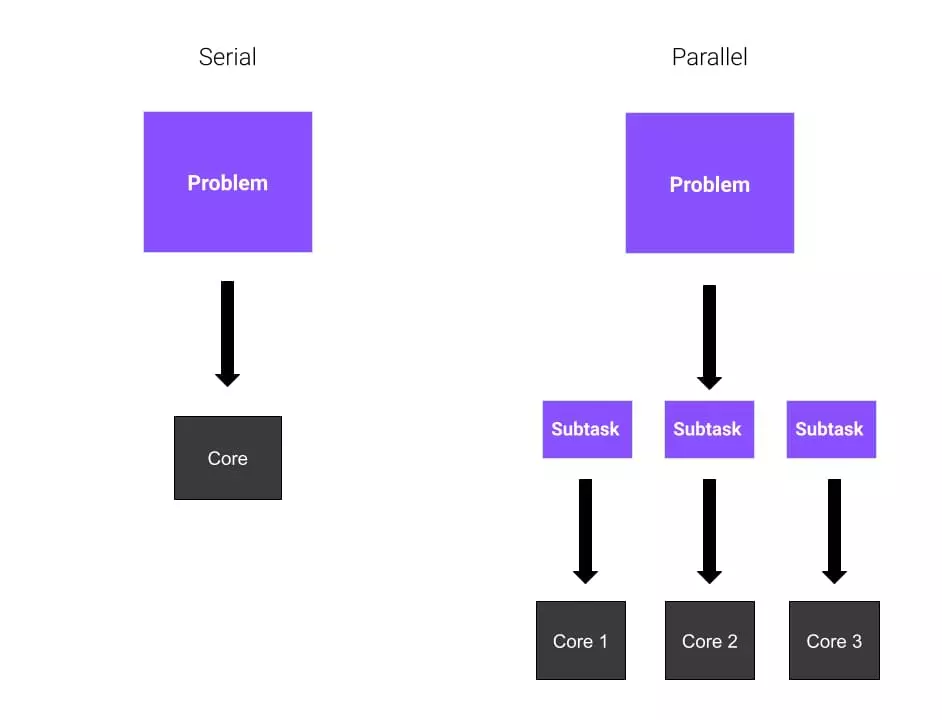
Every tool does the same thing: split the work, run it on separate workers, then collect the results

Big O notation

Big O notation

Runtime growth decides whether parallelism helps

  • Big O notation describes how the runtime grows as the input grows
  • O(1) means constant: reading one array element costs the same whatever the array size
  • O(n) means linear: a single loop takes twice as long when the input doubles
  • O(n²) means quadratic: a nested loop takes four times as long when the input doubles
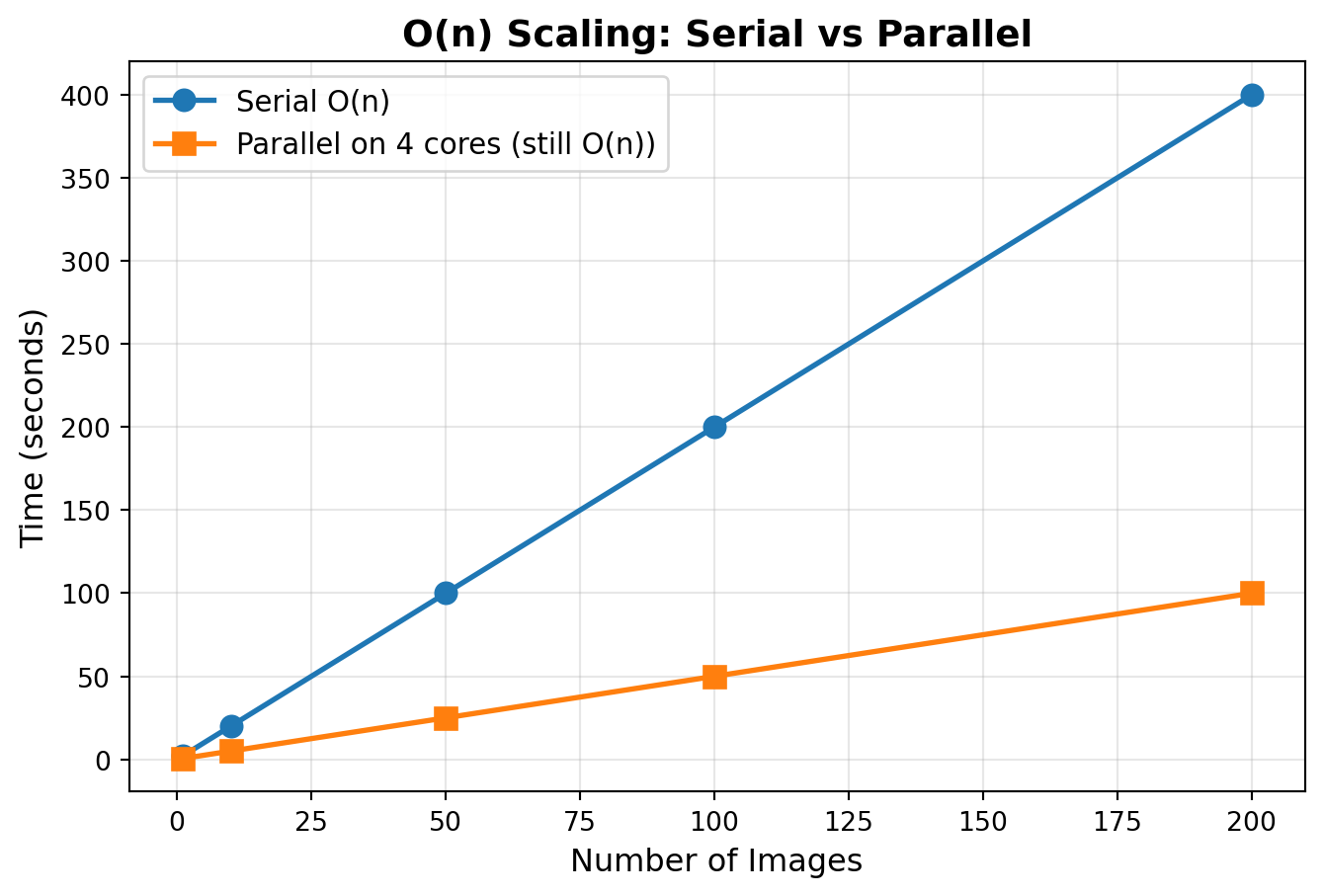
  • Our calculation function called on n inputs is O(n)
  • Two calls take about twice as long as one, and a hundred calls take about a hundred times as long
Code
import matplotlib.pyplot as plt
import numpy as np

# Simulate processing times
num_images = np.array([1, 10, 50, 100, 200])
sequential_time = num_images * 2  # 2 seconds per image
parallel_time = (num_images * 2) / 4  # 4 cores, ideal speedup

plt.figure(figsize=(8, 5))
plt.plot(num_images, sequential_time, 'o-', label='Serial O(n)', linewidth=2, markersize=8)
plt.plot(num_images, parallel_time, 's-', label='Parallel O(n/4)', linewidth=2, markersize=8)
plt.xlabel('Number of Images', fontsize=12)
plt.ylabel('Time (seconds)', fontsize=12)
plt.title('O(n) Scaling: Serial vs Parallel', fontsize=14, fontweight='bold')
plt.legend(fontsize=11)
plt.grid(True, alpha=0.3)
plt.show()
What parallelism does to complexity

  • With p cores, an O(n) problem becomes O(n/p + overhead)
  • Four cores give you close to a 4× saving, minus whatever the coordination costs
  • The best candidates are embarrassingly parallel O(n) tasks
  • Running n independent calculations qualifies
  • Applying the same function to n separate inputs qualifies too
  • What both have in common is no shared state and no dependency between tasks

Parallelism never changes the Big O class. It divides the constant in front of it. An O(n²) algorithm running on eight cores is still an O(n²) algorithm; you only reach “too slow” a little later

  • A poor candidate for parallelism:
# O(n^2): every pair of elements
def pairwise_sum(data):
    n = len(data)
    results = []
    for i in range(n):
        for j in range(n):
            results.append(data[i] + data[j])
    return results

data = list(range(1_000))
print(f"{len(pairwise_sum(data)):,} operations")
1,000,000 operations
  • A thousand elements already means a million operations
  • At n = 100_000 the same code is 10 billion operations, and no core count rescues that
  • Other poor candidates are steps that depend on previous results, algorithms with shared state, and problems limited by memory rather than by the CPU

Try it yourself! 🧠

  1. Install the packages with pip install joblib numpy if you have not done so already
  2. Run the serial version below and write down the time it prints
def square(x):
    return x**2

# Create a large array to process
numbers = np.arange(1000000)

# Sequential version
%timeit [square(x) for x in numbers]
  1. Now run the parallel version and write down its time as well. Be patient: this one takes a while
from joblib import Parallel, delayed

# Parallel version
%timeit Parallel(n_jobs=4)(delayed(square)(x) for x in numbers)
  1. Compare the two times and decide which version you would ship

Appendix 01

Amdahl’s law

Amdahl’s law: the speed-up ceiling

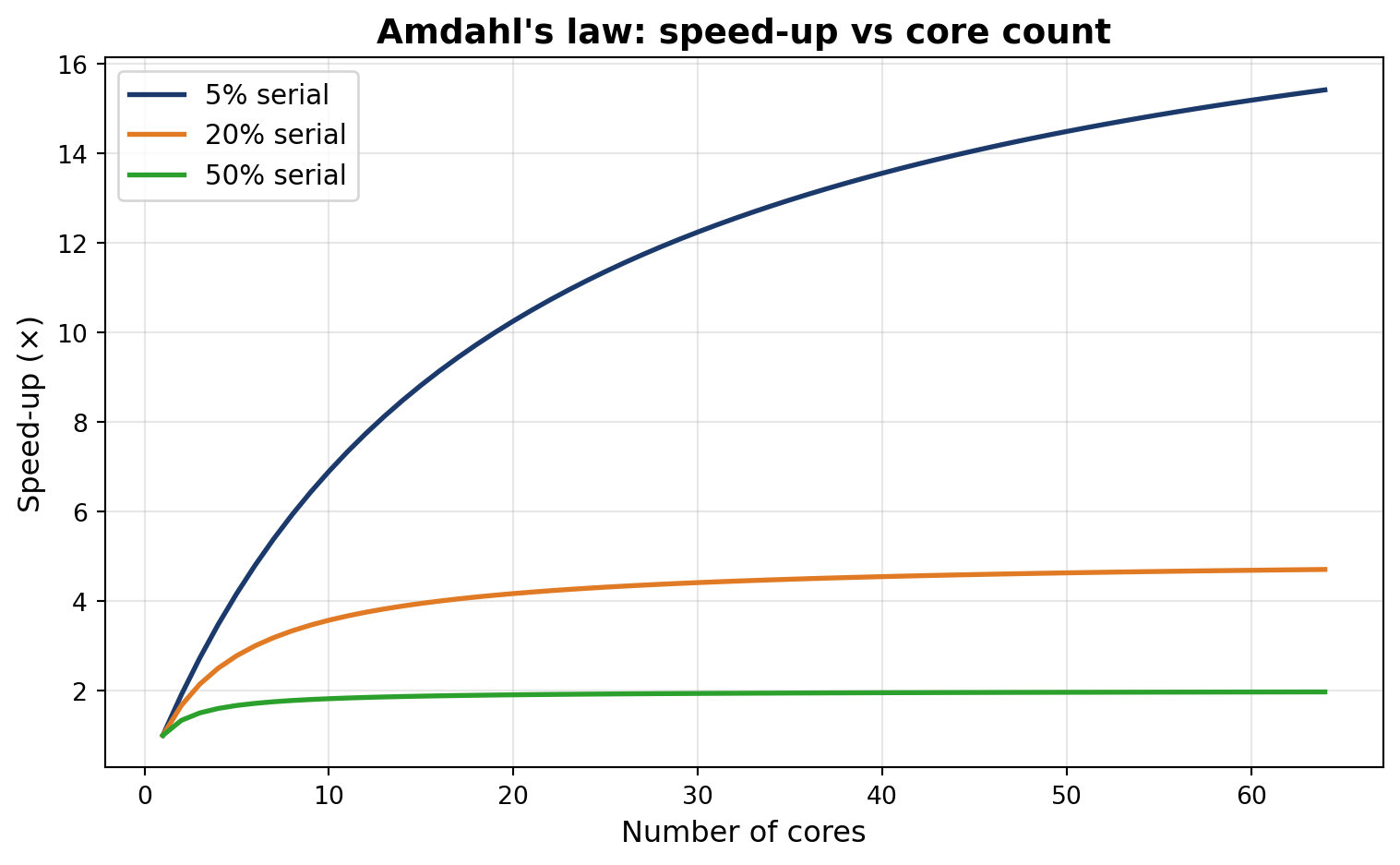
The serial share caps the speed-up

  • Every program has a serial share: the setup, the merging of results, and any step that must wait for the one before it
  • Amdahl’s law says that share caps your maximum speed-up, however many cores you add
  • The formula is \(\text{speedup} = \dfrac{1}{s + \dfrac{p}{N}}\), where \(s\) is the serial fraction, \(p = 1 - s\) is the parallel fraction, and \(N\) is the number of cores
  • Take a program that is 90% parallel, so \(s = 0.1\), running on 8 cores
  • The arithmetic gives \(\frac{1}{0.1 + 0.9/8} = \frac{1}{0.2125} \approx 4.7\times\), well short of the \(8\times\) you might have hoped for
Code
import matplotlib.pyplot as plt
import numpy as np

cores = np.arange(1, 65)
serial_fracs = [0.05, 0.2, 0.5]
labels = ["5% serial", "20% serial", "50% serial"]
colours = ["#1B3A6B", "#E07A24", "#2CA02C"]

plt.figure(figsize=(8, 5))
for s, lab, c in zip(serial_fracs, labels, colours):
    speedup = 1 / (s + (1 - s) / cores)
    plt.plot(cores, speedup, label=lab, linewidth=2, color=c)

plt.xlabel("Number of cores", fontsize=12)
plt.ylabel("Speed-up (×)", fontsize=12)
plt.title("Amdahl's law: speed-up vs core count",
          fontsize=14, fontweight="bold")
plt.legend(fontsize=11)
plt.grid(True, alpha=0.3)
plt.tight_layout()
plt.show()
Global Interpreter Lock (GIL)

The GIL

Why threads do not always help in Python

  • CPython, the Python you are running, has a Global Interpreter Lock (GIL)
  • The GIL lets only one thread execute Python code at a time, however many cores you have
  • Threads still help while your code waits, because the lock is released during downloads and API calls
  • They do nothing while your code computes, because the lock keeps the other threads idle
  • CPU-bound work needs processes: each process is a separate Python with its own GIL
  • NumPy, Polars and DuckDB release the GIL while their C and Rust code runs, so they use all cores with no processes to manage
  • A free-threaded build without the GIL is official since Python 3.14 (PEP 779), but it is not the default
  • How the GIL maps onto the tools you already know:
Task Use Why
Number crunching Processes (joblib, ProcessPoolExecutor) Sidesteps the GIL
Downloading many URLs Threads (ThreadPoolExecutor) GIL released while waiting
NumPy / Polars / DuckDB Either or neither Heavy work runs in C/Rust, outside the GIL
sklearn with n_jobs=-1 Processes (via joblib) Each fold trains independently

Dask

Dask

Familiar pandas code on data bigger than your RAM

  • Dask is a parallel computing library for Python
  • It scales the previous sections to datasets bigger than RAM and to clusters bigger than one machine
  • You write ordinary NumPy and pandas code; Dask handles the parallelism
  • Its task scheduler splits your work into a graph of small tasks and spreads them across your cores
  • Its big data collections are arrays, DataFrames and lists that behave like the ones you know
  • Active development, with a release most months: version 2026.8.0 was released in August 2026
  • Next lecture: when do you actually need Dask, and when does a faster single-machine engine win?

joblib parallelises your functions and leaves the data where it was. Dask chunks the data itself, so a Dask array or DataFrame can be larger than your RAM

Dask arrays

NumPy arrays split into chunks that run in parallel

  • Let’s import Dask and see how it works
import dask.dataframe as dd
import dask.array as da
  • A Dask array is a parallel version of a NumPy array
  • It splits one large array into chunks, and every chunk is an ordinary NumPy array
  • Dask processes those chunks in parallel across your CPU cores
  • You choose the chunk size when you create the array, and here each block is 100 by 100
  • The API matches NumPy, so a.sum(), a.mean() and slicing all work as you expect
  • Let’s build a Dask array from a large NumPy array
  • The Dask array a is a lazy wrapper around the original data, split into 100 by 100 chunks
data = np.random.normal(size=100000).reshape(200, 500)
a = da.from_array(data, chunks=(100, 100))
a
Array Chunk
Bytes 781.25 kiB 78.12 kiB
Shape (200, 500) (100, 100)
Dask graph 10 chunks in 1 graph layer
Data type float64 numpy.ndarray
500 200

Dask arrays

Nothing runs until you call .compute()

  • Dask arrays are lazy, so nothing is computed until you call .compute()
  • That lets you build a full computation graph, an execution plan, before any work starts
  • Dask can then optimise the graph and cut memory use before it executes anything
  • Let’s slice the Dask array a to get the first 10 rows of the sixth column
a[:10, 5] # first 10 rows of the 6th column
Array Chunk
Bytes 80 B 80 B
Shape (10,) (10,)
Dask graph 1 chunks in 2 graph layers
Data type float64 numpy.ndarray
10 1
  • The .compute() method is what finally asks Dask for the numbers
a[:10, 5].compute()
array([-0.47002976,  2.05498662, -1.71513943, -1.48621739,  0.60905255,
       -3.212458  ,  2.42113634, -0.30261545,  2.05459781, -0.61635992])

Dask arrays

  • Dask arrays support most of the NumPy operations you already use
  • Arithmetic works elementwise, so +, *, exp and log behave normally
  • Reductions along an axis work too, including sum(), mean() and std()
a.sum().compute()
np.float64(289.74681304463513)
  • Let’s time the same operation in NumPy on 100 million numbers
size = 100000000
np_arr = np.random.random(size)
%timeit np_result = np.sqrt(np_arr) + np.sin(np_arr)
550 ms ± 117 ms per loop (mean ± std. dev. of 7 runs, 1 loop each)
  • And now the same operation in Dask, with the chunk size left to Dask
da_arr = da.random.random(size, chunks='auto')
%timeit (da.sqrt(da_arr) + da.sin(da_arr)).compute()
385 ms ± 25.8 ms per loop (mean ± std. dev. of 7 runs, 1 loop each)

Not a rule: Dask wins here because sqrt and sin split cacross chunks. On data that fits in memory, building the graph and moving chunks often makes Dask slower. Run %timeit to see the difference

Dask dataframes

Many pandas DataFrames behind one lazy interface

import dask
df = dask.datasets.timeseries()
  • This is a small synthetic dataset of about 240 MB
  • Dask DataFrames are lazy in the same way Dask arrays are
  • Nothing is printed but ellipses, because no rows have been read yet
df
Dask DataFrame Structure:
name id x y
npartitions=30
2000-01-01 string int64 float64 float64
2000-01-02 ... ... ... ...
... ... ... ... ...
2000-01-30 ... ... ... ...
2000-01-31 ... ... ... ...
Dask Name: to_string_dtype, 2 expressions
  • The column names and dtypes are known even so
df.dtypes
name     string
id        int64
x       float64
y       float64
dtype: object

Dask dataframes

Filtering and grouping look exactly like pandas

  • Dask DataFrames support a large subset of the pandas API
  • A few operations, such as head(), display data without being asked
import pandas as pd

pd.options.display.precision = 2
pd.options.display.max_rows = 10

df.head()
name id x y
timestamp
2000-01-01 00:00:00 Jerry 965 -0.30 -0.50
2000-01-01 00:00:01 Victor 1033 0.51 -0.30
2000-01-01 00:00:02 Sarah 1006 -0.76 0.96
2000-01-01 00:00:03 Dan 961 -0.21 0.36
2000-01-01 00:00:04 Ursula 1054 -0.90 -0.73
  • Here we keep the rows where y > 0 and take the standard deviation of x within each group
df2 = df[df.y > 0]
df3 = df2.groupby("name").x.std()
df3
Dask Series Structure:
npartitions=1
    float64
        ...
Dask Name: getitem, 8 expressions
Expr=(((Filter(frame=ArrowStringConversion(frame=Timeseries(dc824a3)), predicate=ArrowStringConversion(frame=Timeseries(dc824a3))['y'] > 0))[['name', 'x']]).std(ddof=1, numeric_only=False, split_out=None, observed=True))['x']
  • Notice that df3 still shows no numbers
  • Calling .compute() runs the plan and hands back a pandas Series
df3.compute()
name
Bob         0.58
Dan         0.58
Edith       0.58
George      0.58
Hannah      0.58
            ... 
Patricia    0.58
Tim         0.58
Ursula      0.58
Victor      0.58
Xavier      0.58
Name: x, Length: 26, dtype: float64

Dask dataframes

.persist() keeps a computed result in memory

  • Aggregations work the same way
  • Here we take the sum of x and the maximum of y within each name
df4 = df.groupby("name").aggregate({"x": "sum", "y": "max"})
df4.compute()
x y
name
Sarah 240.42 1.0
Kevin -117.49 1.0
Alice 117.03 1.0
Patricia 28.00 1.0
Ingrid 192.54 1.0
... ... ...
Norbert -105.56 1.0
Edith 311.77 1.0
Ray 77.46 1.0
Quinn 36.02 1.0
Oliver 257.52 1.0

26 rows × 2 columns

  • If the result fits in RAM, .persist() computes it once and holds it in memory
  • Later computations on persisted data skip the loading and the recomputation
  • Persist a small aggregate, never the raw 240 MB frame you have not filtered yet
df5 = df4.persist()
df5.head()
x y
name
Sarah 240.42 1.0
Kevin -117.49 1.0
Alice 117.03 1.0
Patricia 28.00 1.0
Ingrid 192.54 1.0

Combining Dask and Pandas

The workflow ends with a small pandas DataFrame

  • Dask and pandas are designed to hand work to each other
  • Dask does the heavy lifting over data that will not fit in memory
  • .compute() then returns an ordinary pandas DataFrame for the last few steps
  • Most Dask code reads almost identically to pandas code, so moving between them costs you very little

Load and filter in Dask, aggregate down to something small, call .compute(), then finish in pandas

import dask
import dask.dataframe as dd

df = dask.datasets.timeseries()

# Step 1-2: filter and aggregate with Dask
summary = (
    df[df.x > 0]
    .groupby("name")
    .agg({"x": "mean", "y": "std"})
)

# Step 3: bring to Pandas
pdf = summary.compute()

# Step 4: use Pandas normally
pdf.sort_values("x", ascending=False).head(5)
x y
name
Tim 0.5 0.58
Norbert 0.5 0.58
Kevin 0.5 0.58
Wendy 0.5 0.58
Quinn 0.5 0.58

Try it yourself! 🧠

  1. Install Dask with pip install dask if you have not already
  2. Import numpy and dask.array
  3. Set size = 10_000_000. Use a smaller number if your laptop is short on memory
  4. Build a Dask array of that many random numbers with chunks=100_000
  5. Time da.sqrt(x**2).mean().compute() with %timeit
  6. Repeat steps 4 and 5 with chunks=2_000_000
  7. Repeat them once more with chunks=5_000_000
  8. Write down the three timings before you look at the appendix
import numpy as np
import dask.array as da

size = 10_000_000

# Dask with SMALL chunks
da_data_small = da.random.random(size, chunks=100_000)  # 100 chunks
%timeit da.sqrt(da_data_small**2).mean().compute()

# Dask with MEDIUM chunks
da_data_medium = da.random.random(size, chunks=2_000_000)  # 5 chunks
%timeit da.sqrt(da_data_medium**2).mean().compute()

# Dask with LARGE chunks
da_data_large = da.random.random(size, chunks=5_000_000)  # 2 chunks
%timeit da.sqrt(da_data_large**2).mean().compute()

Read and write data with Dask

Reading and writing data

Thirty daily CSV files from one line of Dask

  • CSV is still the most common format in data science, and for good reasons
  • Pandas reads CSV well, but it loads the entire file into memory first
  • On a large file that can mean several gigabytes of RAM for a question about one column
  • Dask offers a more careful way to read and write CSV
  • The name_function argument below turns one DataFrame into one file per day
  • Writing data/*.csv gives us 30 files for January 2000
df = dask.datasets.timeseries()
df
Dask DataFrame Structure:
name id x y
npartitions=30
2000-01-01 string int64 float64 float64
2000-01-02 ... ... ... ...
... ... ... ... ...
2000-01-30 ... ... ... ...
2000-01-31 ... ... ... ...
Dask Name: to_string_dtype, 2 expressions
import os
import datetime

if not os.path.exists('data'):
    os.mkdir('data')

def name(i):
    return str(datetime.date(2000, 1, 1)
               + i * datetime.timedelta(days=1))

df.to_csv('data/*.csv', name_function=name);

Reading and writing data

One glob pattern reads a whole month

  • The data directory now holds 30 CSV files, one per day in January 2000, and 182 MB in total
  • dd.read_csv takes a glob pattern and treats the whole set as one DataFrame
  • Dask reads the files in parallel and loads only the parts a computation needs
  • Pandas would need all 182 MB in memory before it could answer anything
df = dd.read_csv('data/2000-*-*.csv')
df
Dask DataFrame Structure:
timestamp name id x y
npartitions=30
string string int64 float64 float64
... ... ... ... ...
... ... ... ... ... ...
... ... ... ... ...
... ... ... ... ...
Dask Name: to_string_dtype, 2 expressions
  • Here is a group-by across all 30 files, timed for real
%timeit df.groupby('name').x.mean().compute()
738 ms ± 5.29 ms per loop (mean ± std. dev. of 7 runs, 1 loop each)

Reading and writing data

The same query runs faster on a columnar file

  • CSV works, but newer formats such as Parquet have taken over for analytical work
  • Parquet stores data by column rather than by row, so a query can read one column and ignore the rest
  • It also compresses: the month of CSVs we just wrote is 182 MB, and the same data as parquet is 86 MB
  • That is 53% smaller, on this dataset, with no loss of information
df.to_parquet('data/2000-01.parquet')
  • Reading it back, we can name the columns we want
df = dd.read_parquet('data/2000-01.parquet',
                     columns=['name', 'x'])
df
Dask DataFrame Structure:
name x
npartitions=30
string float64
... ...
... ... ...
... ...
... ...
Dask Name: read_parquet, 1 expression
  • Now the same group-by, on parquet instead of CSV
%timeit df.groupby('name').x.mean().compute()
73.6 ms ± 609 μs per loop (mean ± std. dev. of 7 runs, 10 loops each)

Why Parquet?

Column storage reads only what you ask for

  • CSV is row-based, so reading one column still means scanning every row
  • Parquet is column-based, so it reads the columns you named and skips the others
Feature CSV Parquet
Storage Row-based Column-based
Compression None Snappy/gzip
Column selection Reads all Reads only needed
Data types Text only Typed (int, float, date)
Our January 2000 data 182 MB 86 MB
import pandas as pd

# CSV: reads everything, infers types
df = pd.read_csv("sales.csv")

# Parquet: reads only what you need
df = pd.read_parquet("sales.parquet",
                     columns=["date", "revenue"])

CSV is not obsolete: reach for parquet when you have many columns and query only a few, or when the file passes 100 MB. Stay with CSV for small files, one-off exports, and anything a collaborator will open in Excel

Dask delayed

Dask delayed

A decorator schedules any function you already have

  • Sometimes you do not want a whole Dask DataFrame or Dask array
  • You want to parallelise one function, or one small part of a script
  • dask.delayed does exactly that, and it works on functions you have already written
  • Here are four serial calls to a deliberately heavy function
def calculation(size=10000000):
    arr = np.random.rand(size)
    for _ in range(10):
        arr = np.sqrt(arr) + np.sin(arr)
    return np.mean(arr)

%timeit [calculation() for _ in range(4)]
1.39 s ± 36.7 ms per loop (mean ± std. dev. of 7 runs, 1 loop each)
  • The only change is the @dask.delayed decorator above the function
@dask.delayed
def delayed_calculation(size=10000000):
    arr = np.random.rand(size)
    for _ in range(10):
        arr = np.sqrt(arr) + np.sin(arr)
    return np.mean(arr)

results = []
for _ in range(4):
    results.append(delayed_calculation())

# Compute all results at once
%timeit final_results = dask.compute(*results)
611 ms ± 25.6 ms per loop (mean ± std. dev. of 7 runs, 1 loop each)
  • Nothing in the body of the function changed
  • Calling delayed_calculation() builds a task instead of running one, so dask.compute(*results) is what triggers the work

Dask delayed

Dask draws the plan before running a single task

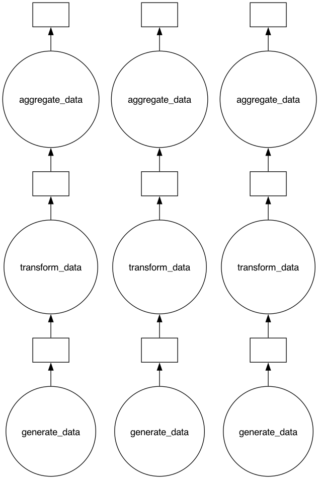
  • Three delayed functions, chained over three input sizes, give us nine tasks in three independent branches
@dask.delayed
def generate_data(size):
    return np.random.rand(size)

@dask.delayed
def transform_data(data):
    return np.sqrt(data) + np.sin(data)

@dask.delayed
def aggregate_data(data):
    return {
        'mean': np.mean(data),
        'std': np.std(data),
        'max': np.max(data)
    }

# Compare execution
sizes = [1000000, 2000000, 3000000]

# Dask execution
dask_results = []
for size in sizes:
    data = generate_data(size)
    transformed = transform_data(data)
    stats = aggregate_data(transformed)
    dask_results.append(stats)

%timeit dask.compute(*dask_results)
27.6 ms ± 323 μs per loop (mean ± std. dev. of 7 runs, 10 loops each)
  • dask.visualize() draws the graph without running any of it
# Needs graphviz twice over: the Python package
# and the binary itself
#   pip install graphviz
#   brew install graphviz   (macOS)
#   apt install graphviz    (Linux)
dask.visualize(*dask_results)

Dask sees all nine tasks before it runs any of them. The three branches never touch each other, so they go to separate workers

The Dask dashboard

Watching the task stream at localhost:8787

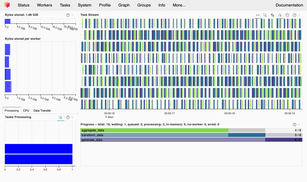
  • Starting a dask.distributed.Client() opens a diagnostics dashboard on port 8787
  • The task stream on the right is the same three-stage pipeline, run in a loop so the picture fills up
  • Each row is one worker thread, and each coloured bar is one task it ran
  • The three colours are generate_data, transform_data and aggregate_data
  • Bars at the same horizontal position in different rows ran at the same moment
  • The dashboard is the fastest way to find out whether your work is actually parallel

White space in a row means that worker had nothing to do. Large gaps usually mean your chunks are too big, so there are fewer tasks than workers

The Dask dashboard at localhost:8787 while this computation ran on my laptop

Best practices

Best practices

Cheaper fixes to try before you parallelise

  • Measure first: %timeit and cProfile will tell you where the time goes, and Amdahl’s law tells you what that share is worth
  • Ask two questions: are the tasks independent of each other, and is each one heavy enough to pay for starting a worker? If either answer is no, do not parallelise
  • Pick the right algorithm: an \(O(n \log n)\) solution beats a parallelised \(O(n^2)\) one on any interesting input
  • Pick the right engine: Polars or DuckDB may finish the job faster than a parallelised pandas, as we will see next lecture
  • Start small: NumPy or pandas may already have a fast function for what you wrote by hand
  • Sample first: ask whether the question really needs all of those terabytes
  • Switch to parquet: the format change alone bought us a large speed-up a few slides ago
  • Call .compute() and .persist() sparingly: every call triggers execution, so batch the work into one
  • Experiment with chunk sizes: try a few by hand, or start from chunks='auto'
  • The Dask team keeps a longer list at Dask best practices

The mistake I see most often: students parallelise before they profile. Run %timeit first. If the hot spot turns out to be disk reads or an \(O(n^2)\) loop, more cores will not save you, and you will have spent an afternoon finding that out

Summary

What we learned today

  • Serial and parallel execution: map, embarrassingly parallel problems, and joblib for the easy cases
  • concurrent.futures ships with Python: ProcessPoolExecutor for CPU work, ThreadPoolExecutor for waiting
  • Big O notation: parallelism cuts the constant factor and leaves the complexity class alone
  • Amdahl’s law: the serial share caps your speed-up, so measure it before you buy cores
  • The GIL: threads help while Python waits, processes help while Python computes, and NumPy sidesteps both
  • Dask gives you lazy arrays and DataFrames for data bigger than RAM
  • dask.delayed parallelises functions you have already written, and dask.visualize shows the plan
  • Parquet cut our January 2000 data from 182 MB to 86 MB and made the group-by much faster
  • Next lecture, Scaling Data Analysis in Practice, puts Polars and DuckDB against pandas and Dask on the WDI panel. They use every core by default, with nothing to configure
Engine Language Parallel? Out-of-core?
pandas Python/C Single-threaded No
Polars Rust All cores Yes (streaming)
DuckDB C++ All cores Yes
Dask Python All cores + clusters Yes

Thank you! 😊

Appendix 01

Solution to the joblib exercise

  • Here is the solution to the exercise
def square(x):
    return x**2

# Create a large array to process
numbers = np.arange(1000000)

# Sequential version
%timeit [square(x) for x in numbers]
44.8 ms ± 475 μs per loop (mean ± std. dev. of 7 runs, 10 loops each)
from joblib import Parallel, delayed

# Parallel version
%timeit Parallel(n_jobs=4)(delayed(square)(x) for x in numbers)
1.98 s ± 24.2 ms per loop (mean ± std. dev. of 7 runs, 1 loop each)
  • Expected result: the parallel version is slower here. square(x) finishes so fast that joblib’s process-spawning overhead swamps the work. Parallel computing pays off when each task is heavy

Back to exercise

Appendix 02

Chunk sizes compared

  • Ten million random numbers, computing mean(sqrt(x^2)) at four chunk sizes
  • The middle setting wins on my laptop, and the timings below say by how much
size = 10_000_000

# Dask with SMALL chunks  # 100 chunks
da_data_small = da.random.random(size, chunks=100_000)
%timeit da.sqrt(da_data_small**2).mean().compute()
45.1 ms ± 503 μs per loop (mean ± std. dev. of 7 runs, 10 loops each)
# Dask with MEDIUM chunks  # 5 chunks
da_data_medium = da.random.random(size, chunks=2_000_000)
%timeit da.sqrt(da_data_medium**2).mean().compute()
15.5 ms ± 1.11 ms per loop (mean ± std. dev. of 7 runs, 100 loops each)
# Dask with LARGE chunks  # 2 chunks
da_data_large = da.random.random(size, chunks=5_000_000)
%timeit da.sqrt(da_data_large**2).mean().compute()
21.3 ms ± 298 μs per loop (mean ± std. dev. of 7 runs, 10 loops each)
# Dask with AUTO chunks  # Dask picks
da_data_auto = da.random.random(size, chunks='auto')
%timeit da.sqrt(da_data_auto**2).mean().compute()
32.7 ms ± 1.35 ms per loop (mean ± std. dev. of 7 runs, 10 loops each)

Back to exercise