DATASCI 350 - Data Science Computing

Lecture 10 - Reproducible Research and Literate Programming

Danilo Freire

Department of Data and Decision Sciences
Emory University

Nice to see you all again! 😊

Recap of our last lectures

Before the quiz, we covered

  • The command line: navigation, file management, text tools, pipes, and scripts
  • Git: repositories, staging, commits, branches, and merges
  • GitHub: remotes, forks, pull requests, issues, and the gh CLI
  • Last class you put all of it to work in quiz 01
  • Congratulations, that was the hardest setup work of the course 🎉
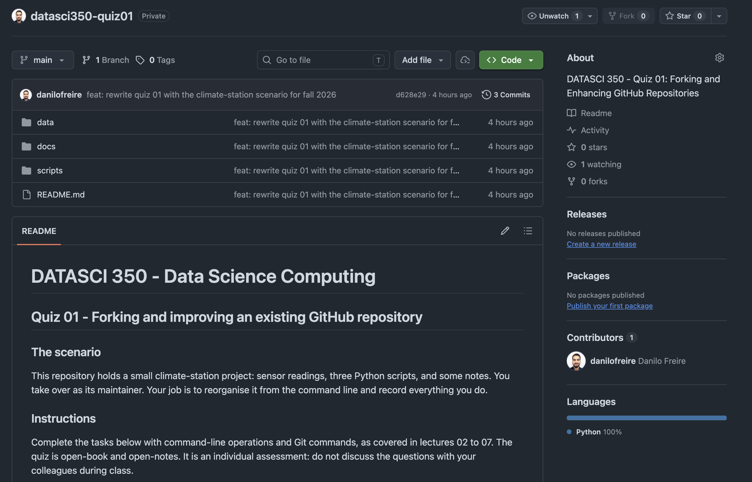
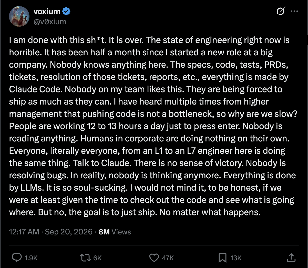
I hope the image doesn’t bring back bad memories! :)

Today’s lecture

Today we start a new module, and a new question: can anyone check your work?

  • The reproducibility crisis: why so much published research fails when someone re-runs it
  • The habits that prevent it: project structure, raw data, paths, seeds, environments
  • Literate programming: text, code, and results in one file, so they cannot drift apart
  • Quarto, the tool we will use for it: installing it and writing your first document
  • Next class: PDFs, citations, websites, and reports that write themselves

Why is reproducible research so important? 🤔

The reproducibility crisis

  • Reproducibility: someone else, using your data and code, can get the same results you got
  • Sounds like a low bar. Across many fields, a large share of published findings fail it
  • This is the reproducibility crisis. Psychology, medicine, and economics were hit hardest, but no empirical field escaped
  • The usual suspects: small samples, p-hacking, selective reporting, and code that is never shared
  • Our focus in this course: code and data. Most computational results fail for a mundane reason, as you will see in a minute

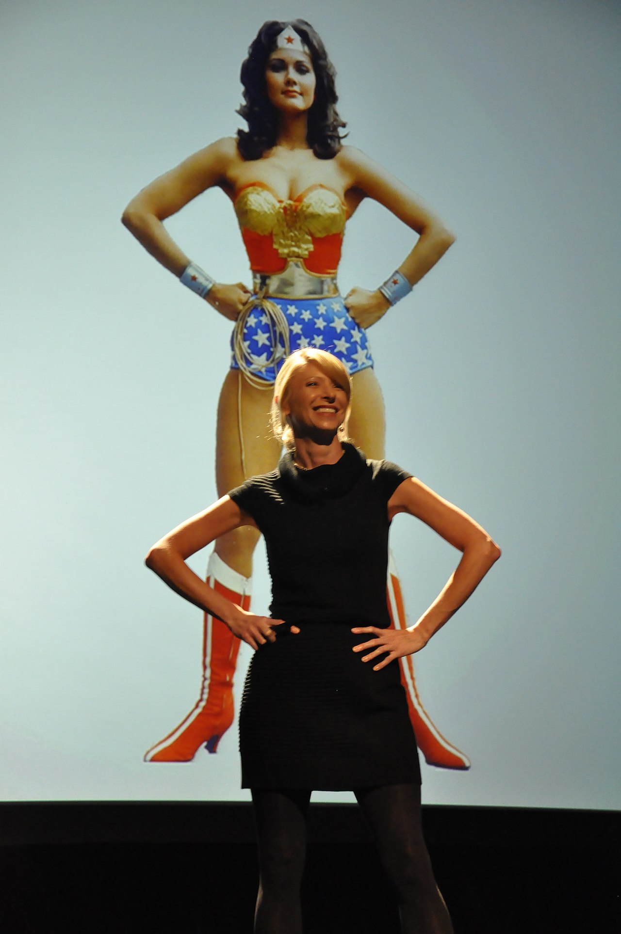
Amy Cuddy’s “power posing” theory. 78 million TED Talk views, but it could never be replicated

How bad is it? Two famous papers

Medicine
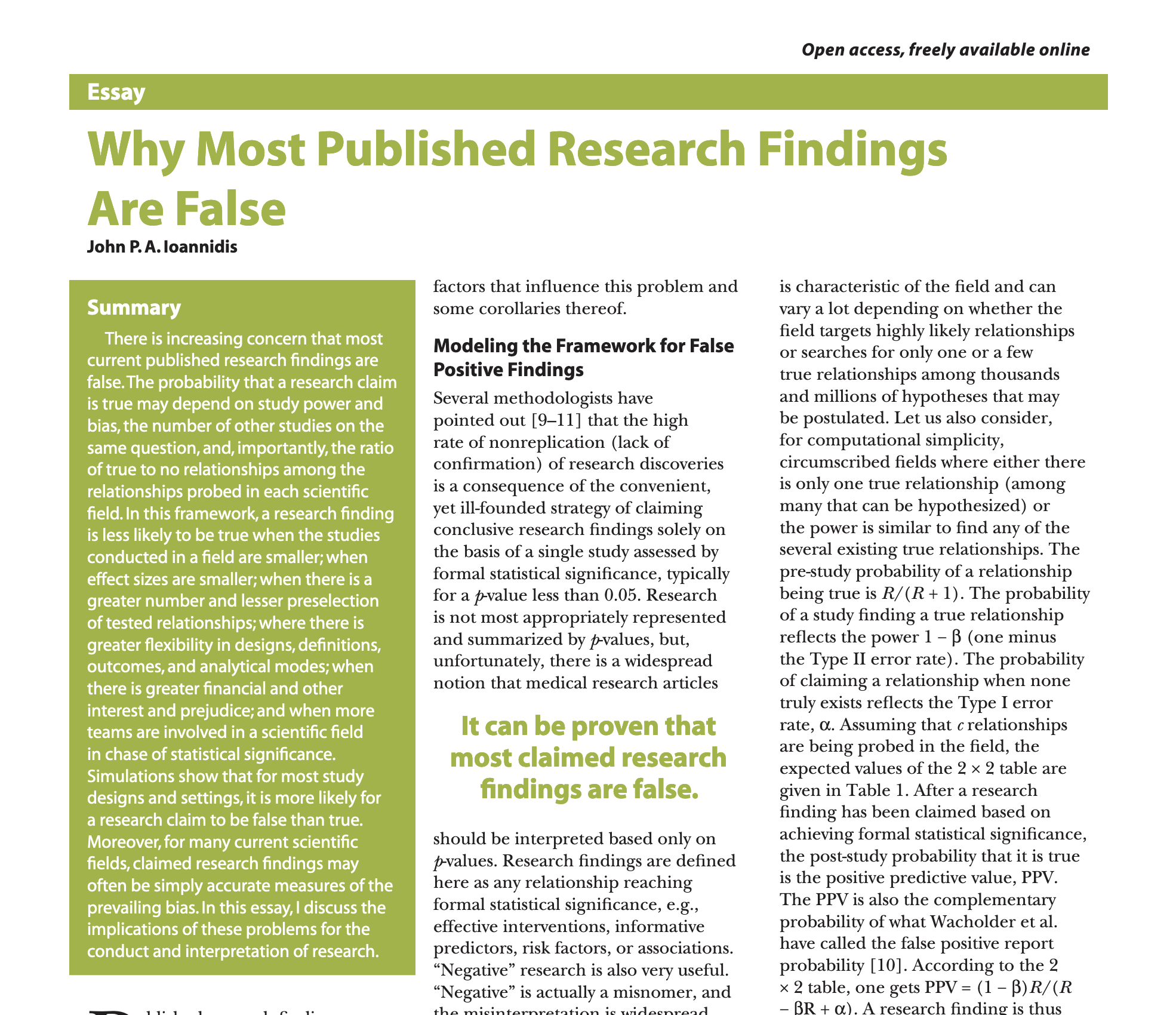
  • Ioannidis (2005), one of the most cited papers in medicine
  • Argument: for most study designs, a positive finding is more likely to be false than true
  • Why: small samples, flexible analyses, financial interests, many teams racing on the same question

Psychology

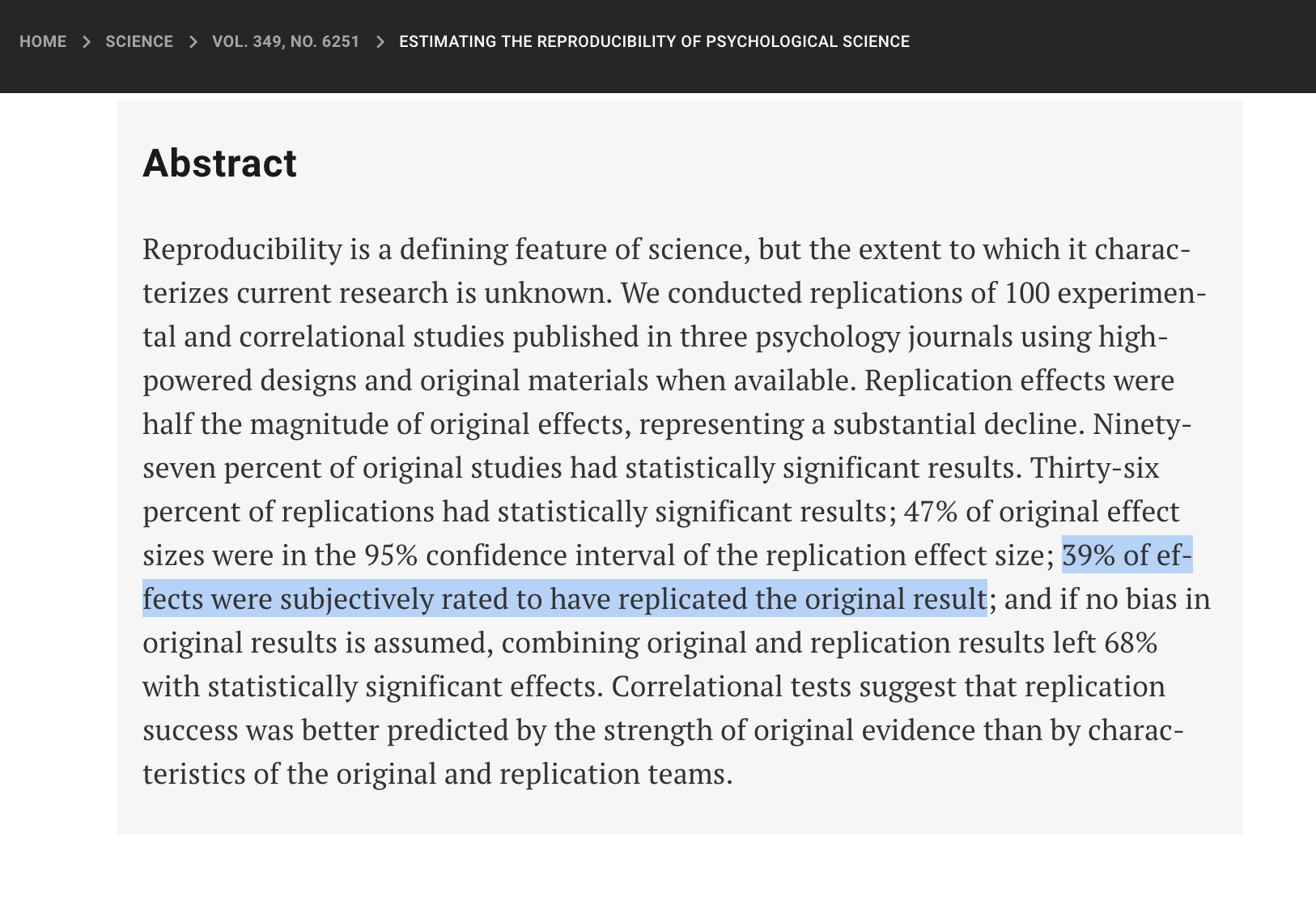
  • Open Science Collaboration (2015): 270 researchers re-ran 100 published psychology experiments
  • Originals: 97% significant. Replications: 36% significant, with effect sizes cut in half
  • The fallout changed journal policy: pre-registration, open data, registered reports

We all write code, so we are fine, right?

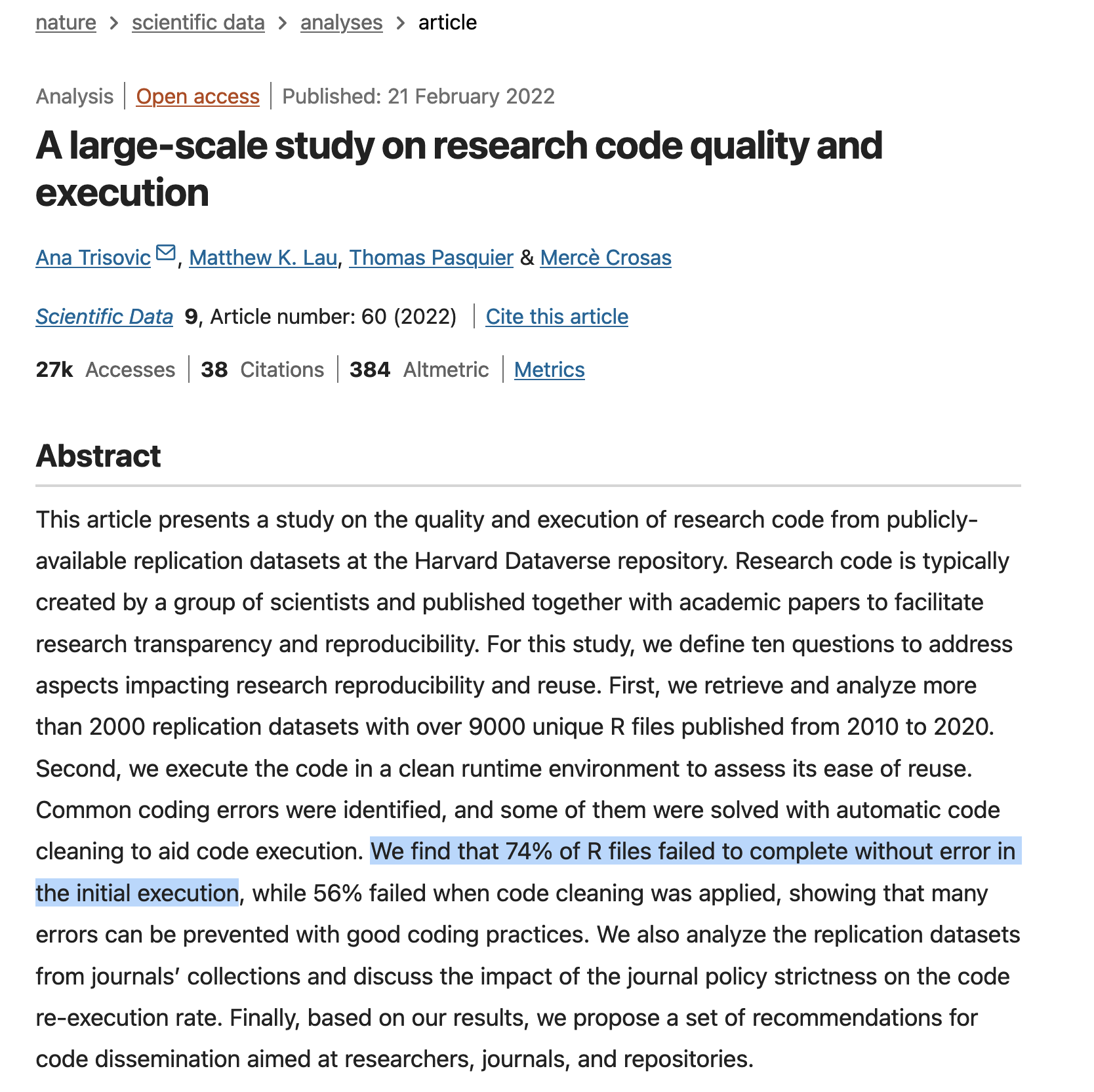
  • Trisovic et al. (2022) downloaded 2,109 R files from Harvard Dataverse and tried to run them
  • 74% produced errors on the first attempt. After automated fixes, 56% still failed
  • The reasons are not exotic: missing packages, hardcoded paths, functions that changed, data left out of the repository
  • These are files that authors chose to deposit alongside their publications
  • If the code people publish on purpose does not run, imagine the code they do not publish 😅

Five selfish reasons to work reproducibly

So far this sounds like a duty to science. Markowetz (2015) argues you should do it for yourself:

  1. It helps you avoid disaster: you catch your own errors before a reviewer, a retraction, or a job interview does
  2. It makes writing easier: when the data changes, every number and figure in the paper regenerates itself
  3. It helps reviewers see it your way: they can run your analysis instead of guessing what you did
  4. It gives your work continuity: a new collaborator, or future-you, can pick the project up tomorrow
  5. It builds your reputation: working, shared code is public proof that you know what you are doing

Reason 2 alone will save you hours in this course. And keep reason 1 in mind: in a few slides you will meet two famous economists who needed it

What does it take to be reproducible?

The reproducibility ladder

  • People use four words for this, and they mean different things
  • Re-runnable: the code runs again on your machine, today
  • Reproducible: same code, same data, same results, on anyone’s machine
  • Replicable: new data, collected independently, gives the same finding
  • Reusable: others can apply your work to their own questions
  • Each step is harder than the one below it
  • Replicability depends on data you may never get, so it sits mostly outside your control

Reproducibility is entirely within your control, and that is why this course grades you on it

harder

easier

reusable

replicable

reproducible

re-runnable

Most published work does not clear the first step

The four ingredients

A result is reproducible only if all four of these travel together:

  1. Code: every step from raw data to final number, written down and runnable
  2. Data: the raw inputs, or a script that fetches them
  1. Environment: the language and package versions the code needs
  2. Documentation: what the project does, and the order to run things in

Each one fails on its own:

  • Code without data: readers can admire your work, but they cannot check it
  • Code and data without the environment: it runs today and breaks next year
  • All three without documentation: nobody knows which script to run first
  • Miss one ingredient and the result is not reproducible

Project structure

  • One folder per project, and the same layout in every project, so you never wonder where a file goes
  • We will use this one for the rest of the course, and the final project requires it
my-project/
├── data/
│   ├── raw/          # never edited by hand
│   └── clean/        # built by scripts
├── scripts/          # the code, in run order
├── output/           # figures and tables
└── README.md         # what and how
  • The layout separates inputs from outputs: data/raw/ holds what you collected, and everything else can be rebuilt from it
  • data/raw/ is read-only: download the files once and never touch them again
  • Numbered scripts (01-clean.py, 02-analyse.py) make the run order part of the name
  • data/clean/ and output/ are disposable: delete them and the scripts bring them back
  • Generated files often stay out of Git: put data/clean/ and output/ in .gitignore and commit only sources
  • README.md explains the project to the next person, who is usually you in six months

If you deleted everything except data/raw/ and scripts/, could you rebuild the project?

Every project needs a README

  • You have been reading READMEs all term: GitHub shows one on every repository page
  • A good one answers three questions: what is this, how do I rebuild it, and in what order
  • List each data source and the date you downloaded it, so stale data is easy to spot
  • List the commands that rebuild the project, in run order, ready to copy and paste
  • Note the language and package versions (more on those in a minute)
  • Ten lines are enough. Write it while the project is small, and keep it current as the project grows
# Rainfall and crop yields in Brazil

Analysis of rainfall and maize yields, 2000-2024.

## Data
- data/raw/rainfall.csv: INMET, downloaded 12 Sep 2026
- data/raw/yields.csv: IBGE, downloaded 12 Sep 2026

## How to rebuild
Run the scripts in order:

    python scripts/01-clean.py
    python scripts/02-analyse.py
    quarto render report.qmd

## Environment
Python 3.13, pandas 3.0, matplotlib 3.10

The most famous spreadsheet error in economics

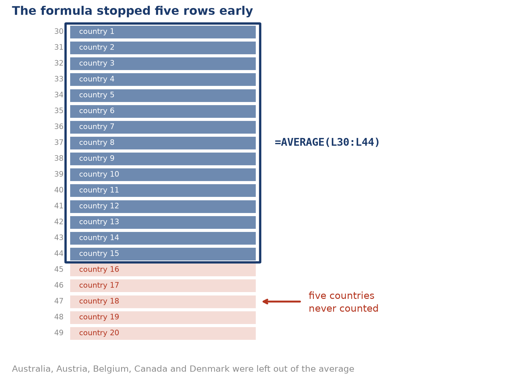
  • Reinhart and Rogoff (2010), “Growth in a Time of Debt”: above 90% debt-to-GDP, growth turns negative
  • After 2008, it became the standard citation for austerity
  • In 2013, a graduate student, Thomas Herndon, could not reproduce it, and asked for the spreadsheet
  • One formula averaged rows 30 to 44, not 30 to 49, dropping five countries
  • Corrected, growth above the threshold was +2.2%, not -0.1%
  • Three years of policy debate passed before anyone noticed, because the analysis sat in a private spreadsheet
  • A public script and dataset would have caught it in an afternoon!

The absolute path problem

The single most common reason code fails on another machine:

analysis.py
import pandas as pd

df = pd.read_csv("/Users/ana/Desktop/project/data/raw/rainfall.csv")

Anyone else who runs it gets:

FileNotFoundError: [Errno 2] No such file
or directory:
'/Users/ana/Desktop/project/data/raw/rainfall.csv'
  • An absolute path starts at the root (/) and names one exact spot on one exact machine
  • Only Ana has a /Users/ana. The script fails everywhere else, however good the rest of the code is
  • A relative path starts from the working directory instead, the same idea as pwd in the shell
  • Every running program has one, inherited from wherever you launched it
  • Which is why “it works when I run it” proves very little

Hardcoded paths were among the top causes of failure in the Trisovic study. The fix costs nothing

Relative paths fix it

Write paths relative to the project folder, and the project works anywhere:

analysis.py
import pandas as pd

df = pd.read_csv("data/raw/rainfall.csv")

Use pathlib when you need to build paths safely across operating systems:

analysis.py
from pathlib import Path

raw = Path("data") / "raw" / "rainfall.csv"
df = pd.read_csv(raw)
  • pathlib handles the separator for you, so the same line works on macOS, Linux, and Windows
  • Quarto renders each document relative to the folder holding the .qmd file, which is usually what you want
  • Avoid os.chdir(). It changes state halfway through a script and makes the rest of the file hard to follow

If your code contains your username, it is not reproducible

Randomness needs a seed

Run this twice, get two answers, and the numbers in your report change on every render:

import numpy as np

print(np.random.normal(size=3).round(3))
[ 0.567 -0.359  0.094]
[ 2.073 -0.402  1.267]

Set a seed first and the sequence is fixed, so anyone running your code gets exactly what you got:

np.random.seed(350)
print(np.random.normal(size=3).round(3))

np.random.seed(350)
print(np.random.normal(size=3).round(3))
[ 1.697 -0.533 -0.311]
[ 1.697 -0.533 -0.311]
  • Computers cannot produce true randomness
  • np.random is a pseudorandom generator: a formula that walks through a fixed sequence of numbers
  • The seed picks where that walk starts, which fixes the whole sequence in advance
  • Newer code makes the generator an explicit object:
rng = np.random.default_rng(350)
rng.normal(size=3)
  • Every library keeps its own generator. Python’s random and scikit-learn’s random_state= need seeding separately
  • Randomness hides in sampling, train-test splits, and the starting weights of most models
  • If a number came from a random draw, seed it

Record your environment

  • Packages change. A function gains an argument, a default flips, a method is removed
  • Code that worked in 2024 can give different numbers in 2026, or refuse to run at all. This is called version drift
  • The fix is to record what you used, so the next person can match it

At minimum, note the versions in your README:

import sys, numpy, pandas

print("python:", sys.version.split()[0])
print("numpy :", numpy.__version__)
print("pandas:", pandas.__version__)
python: 3.13.13
numpy : 2.4.3
pandas: 3.0.2

You can also ask pip for the full list:

Terminal
pip list
Package         Version
--------------- -------
jupyter_client  8.6.3
matplotlib      3.10.8
numpy           2.4.3
pandas          3.0.2

A version list helps the next person diagnose a failure. Module 08 adds the tools that prevent one: virtual environments, uv, and containers. Until then, write the versions down

Literate programming

Literate programming

  • So far, habits. Now a tool that enforces the biggest one: text, code, and results in one file
  • Donald Knuth coined literate programming in 1984: write for humans first, machines second
  • Two operations pull the file apart:
    • Weaving: the readable document (HTML, PDF)
    • Tangling: the executable code
  • Explaining what you are doing catches bad logic before it reaches your results
  • The numbers come from the code, so they cannot go stale
From LaTeX to Quarto

  • LaTeX came first. Beautiful output, verbose syntax, steep learning curve (I know, I’ve been there 😅)
  • Markdown kept the ideas and dropped the ceremony: **bold**, - list, [link](url)
  • R Markdown added executable chunks for R, and Jupyter did the same for Python
  • Each is fine alone. Mixing languages or output formats is where they struggle
  • Quarto (2022, by Posit) rebuilt R Markdown to be language-agnostic: Python, R, Julia, Observable JS
  • One .qmd renders to HTML, PDF, Word, slides, websites, books, and dashboards
  • Pandoc does the final conversion underneath
  • These slides, the course website, and every course PDF are Quarto. Learn it once, use it everywhere

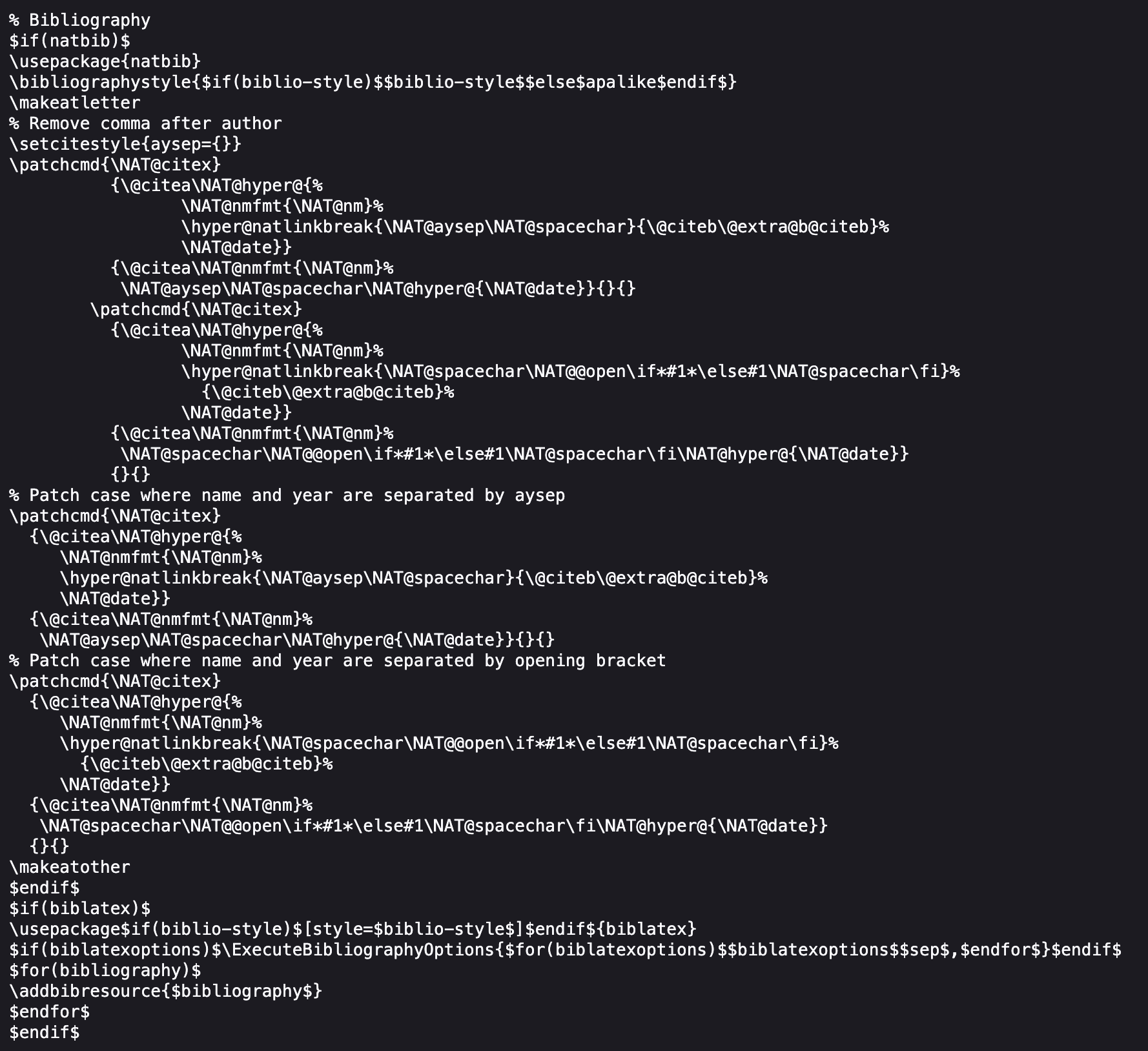
Part of a LaTeX template. This is why Markdown happened

What Quarto can produce

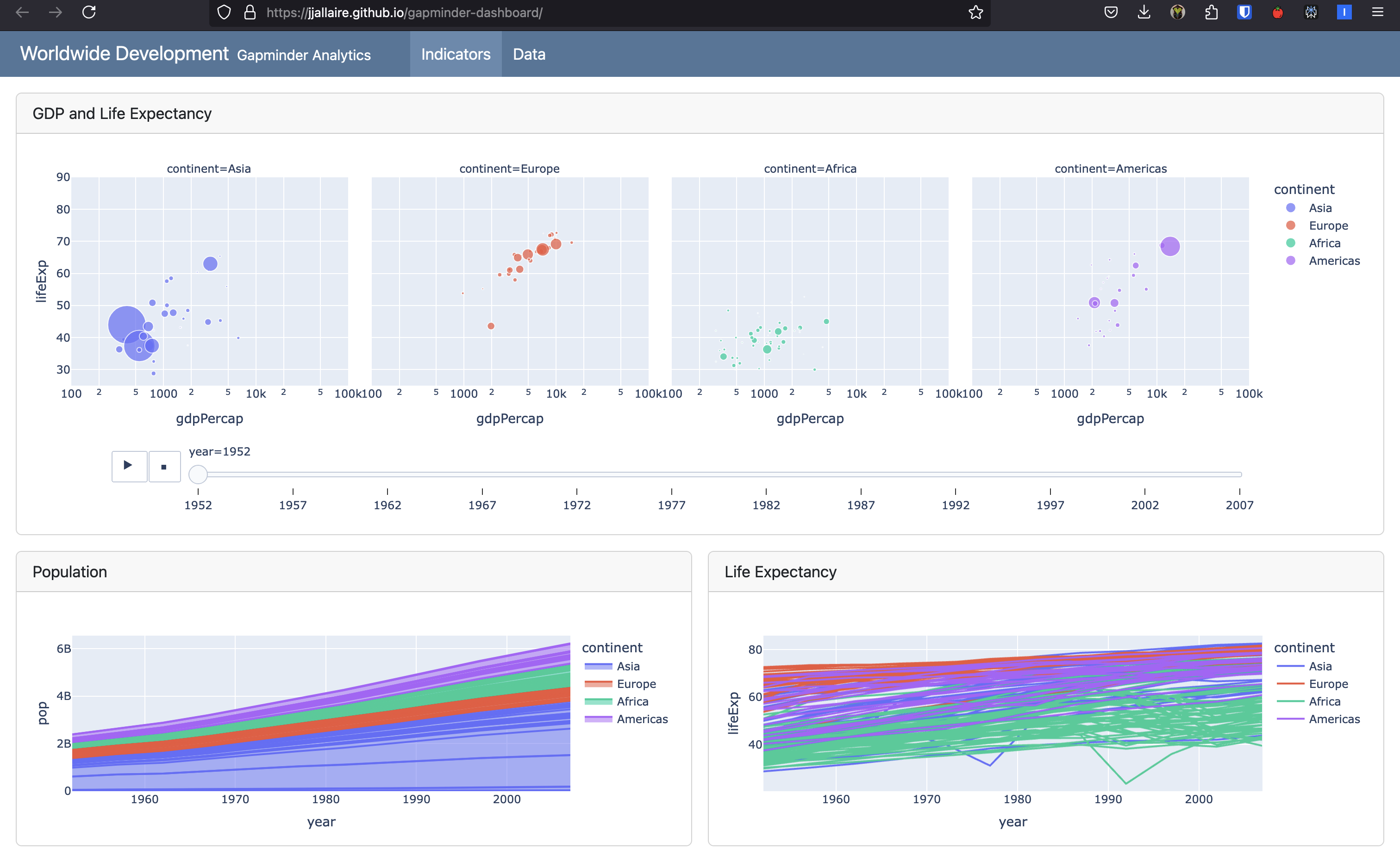
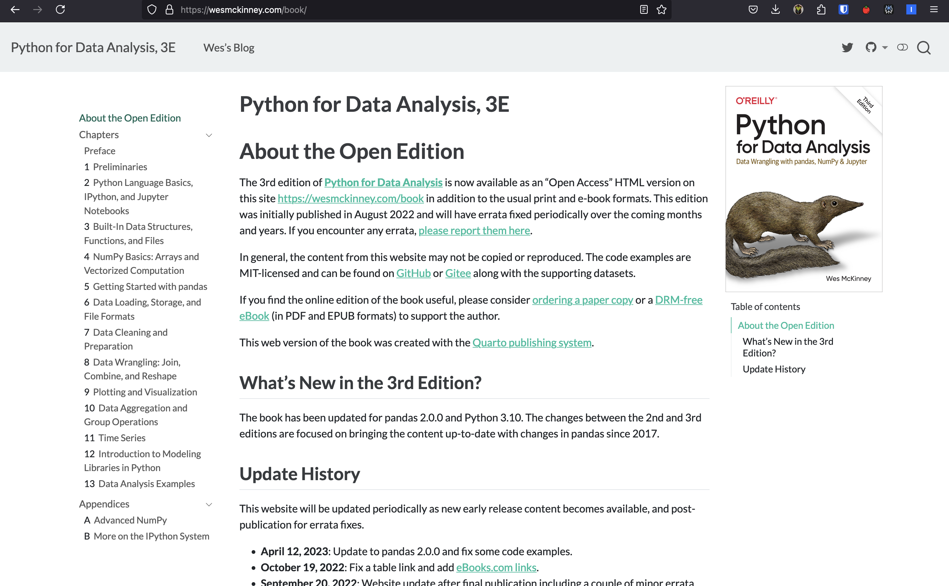
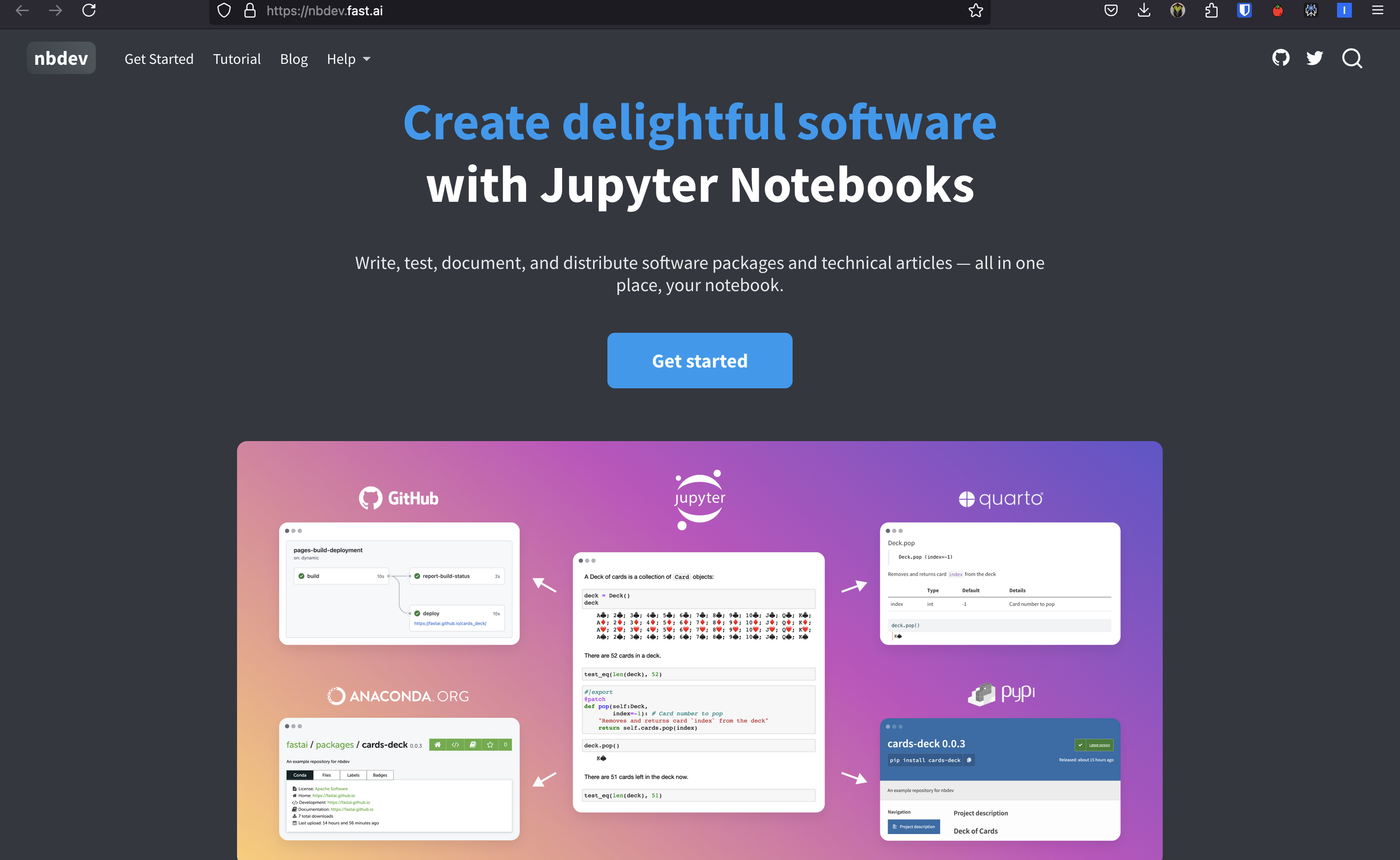
  • Clockwise from top left: a company report, an interactive dashboard, a website, and a book
  • All four are plain text files, so all four live happily in Git
  • Same source, same commands, different format: line
  • Click any image to zoom in

How does Quarto work?

%%{
  init: {
    "theme": "dark",
    "themeCSS": ".label foreignObject, .cluster-label foreignObject { font-size: 90%; overflow: visible; }"
  }
}%%
flowchart LR
  A1[qmd] --> C{"knitr<br>(R)"}
  A1[qmd] --> B{"Jupyter<br>(Python)"}
  A2[ipynb] --> B{"Jupyter<br>(Python)"}
  B --> D[md]
  C --> D[md]
  D --> E{Pandoc}
  E --> F[pdf]
  E --> G[docx]
  E --> H[html]
  E --> I[...]

  subgraph engine [Engine]
  B
  C
  end

  • Quarto files use the .qmd extension, but you can also feed Jupyter notebooks (.ipynb) straight into Quarto with some YAML configuration
  • The pipeline: .qmd → engine (Jupyter or knitr) → .mdPandoc → final output
  • Pandoc handles the last step: it reads Markdown and writes HTML, PDF, Word, and dozens of other formats
  • You rarely interact with Pandoc directly. Quarto calls it for you, passing the options from your YAML header

Getting Quarto running 🛠️

Installing Quarto

  • Download the installer for your system from the page on the left, or use a package manager
  • On macOS, Homebrew does it in one line:
Terminal
brew install --cask quarto
  • On Windows, install Quarto inside WSL so it lives next to your shell and Git
  • To render PDFs you also need LaTeX. Install the lightweight TinyTeX and you are done:
Terminal
quarto install tinytex

Did it work? Ask Quarto itself

Terminal
quarto check
Quarto 1.9.38
[✓] Checking environment information...
[✓] Checking versions of quarto binary dependencies...
      Pandoc version 3.8.3: OK
      Dart Sass version 1.87.0: OK
[✓] Checking Quarto installation......OK
      Version: 1.9.38
[✓] Checking tools....................OK
      TinyTeX: v2026.04
[✓] Checking LaTeX....................OK
[✓] Checking basic markdown render....OK
[✓] Checking Python 3 installation....OK
      Version: 3.13.13
      Jupyter: 5.9.1

Run this first whenever something stops working. Your version numbers will differ from mine, and that is fine

Write in whatever editor you like

  • A .qmd file is plain text. VS Code, RStudio, Jupyter Lab, Neovim, or Notepad: they all work
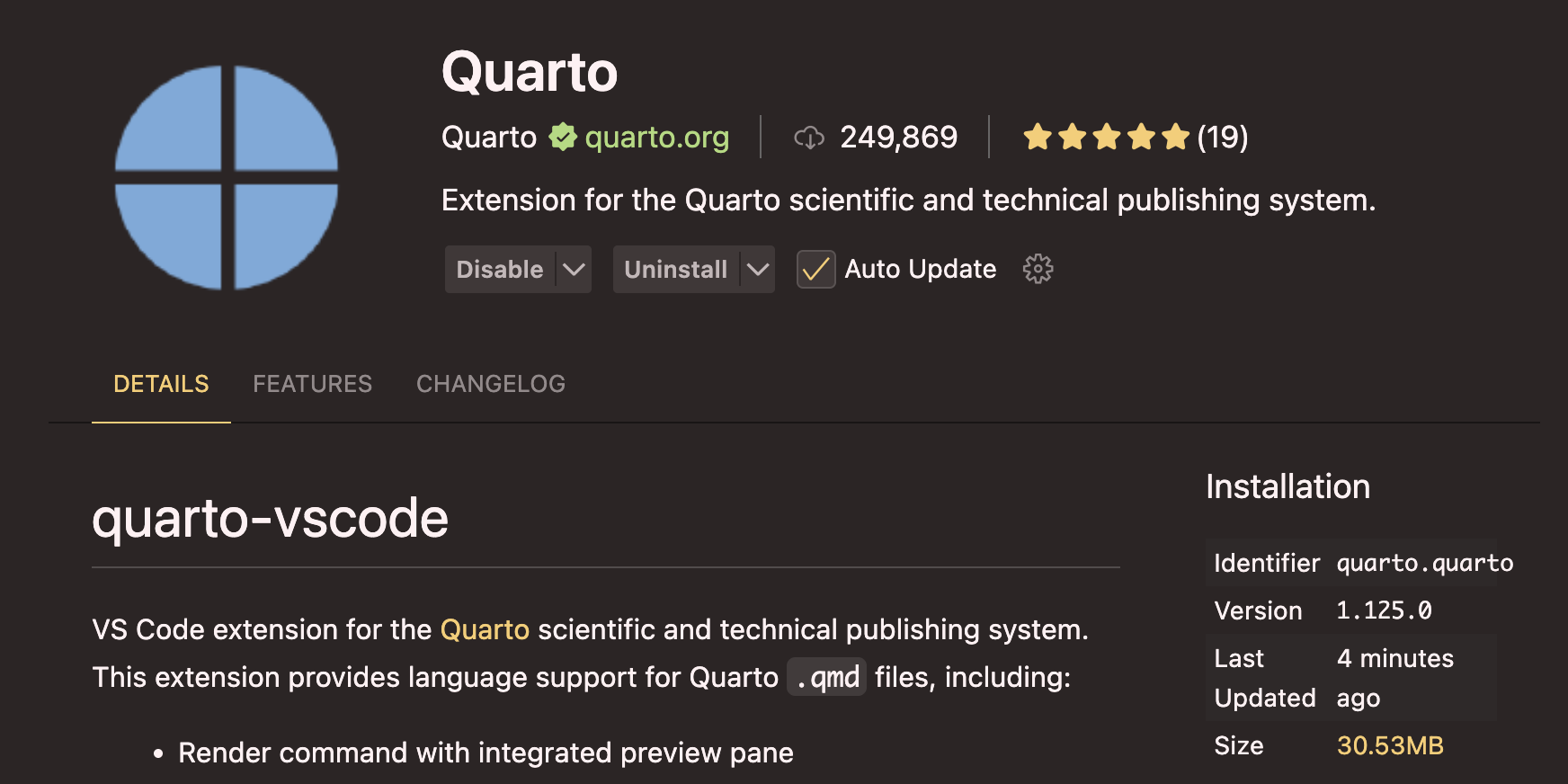
  • We will use VS Code with the Quarto extension: syntax highlighting, completion, a render button, and a live preview
  • Install it from the Extensions marketplace, like the extensions you already have
  • It also offers a visual editor, which renders the Markdown as you type. Try both and keep the one you like

Two commands you will use every day

Of course, there is a CLI for that! Quarto has several commands (quarto --help lists them), but two do almost all the work:

Terminal
## Render a file to its default format
quarto render report.qmd

## Render to a specific format
quarto render report.qmd --to pdf

## Render, open in the browser, and re-render on every save
quarto preview report.qmd
  • render builds the document once. Use it when you are done
  • preview keeps a live version open while you write. Use it the rest of the time
  • The output lands next to the source file: report.qmd becomes report.html

Your first Quarto document

Anatomy of a Quarto document

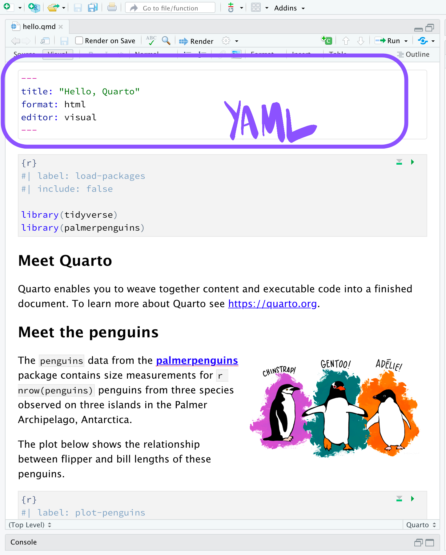
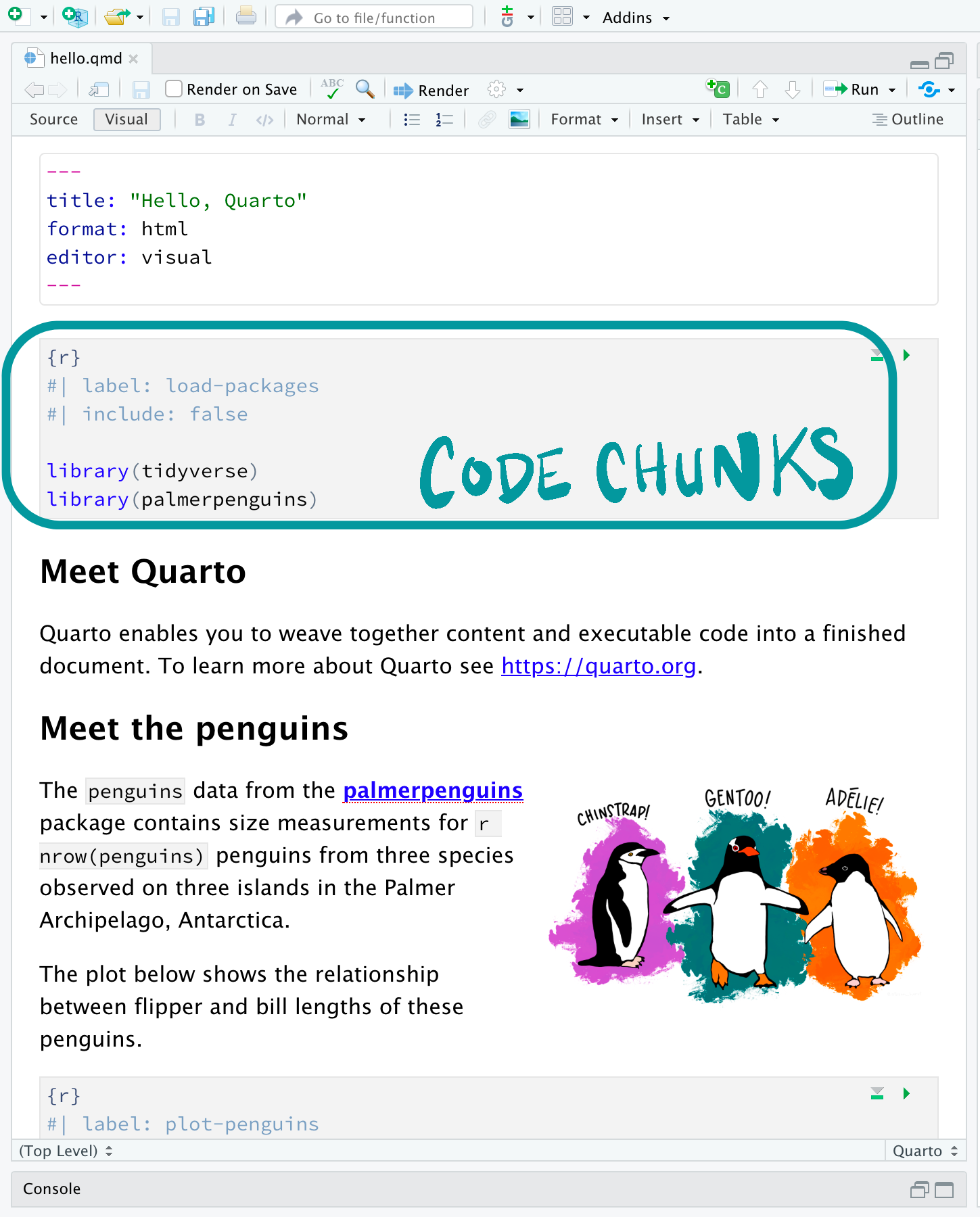
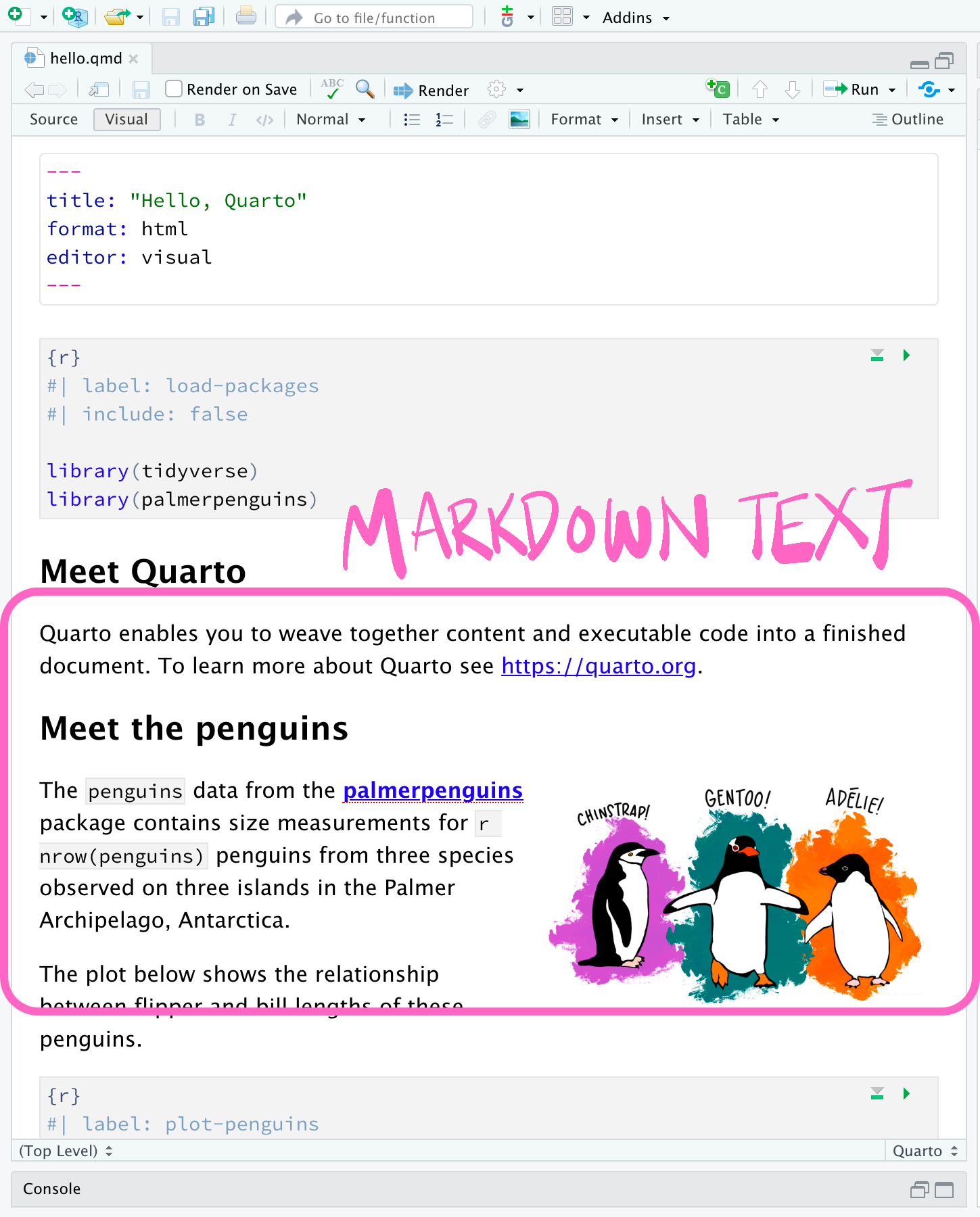
  • A Quarto document contains three types of content: a YAML header, code chunks, and Markdown text
  • That is the whole format. Let’s look at each part in turn (Markdown in depth comes next lecture)

The YAML header

---
title: "Rainfall report"
author: "Your name"
date: 2026-10-06
format:
  html:
    toc: true
    code-fold: true
execute:
  warning: false
jupyter: python3
---
  • YAML stands for “YAML Ain’t Markup Language”, a recursive joke. It describes data, not documents
  • Sits at the very top, between two lines of three dashes (---)
  • key: value pairs, where indentation creates nesting. Use spaces: tabs are illegal in YAML
  • format: html is the short form. Indent underneath it to pass options, as on the left
  • execute: sets defaults for every chunk in the document
  • Quote any value containing a colon: title: "Quarto: a first look"
  • The same syntax runs _quarto.yml, GitHub Actions, and Docker Compose. Learn it once

Code chunks

```{python}
#| label: fig-rainfall
#| echo: false
#| warning: false

import matplotlib.pyplot as plt

plt.bar(rain["month"], rain["mm"])
plt.ylabel("Rainfall (mm)")
plt.show()
```
  • Three backticks and {python} open a chunk; three backticks close it
  • When you render, the chunk runs, and its output lands in the document
  • Lines starting with #| are chunk options, in YAML style:
    • echo: false hides the code, keeps the output
    • eval: false shows the code, skips running it
    • warning: false hides warnings
    • label names the chunk, so you can cross-reference figures

The chunk options you will use most

Option Effect
echo: false hide the code, keep the output
eval: false show the code, do not run it
include: false run the code, show nothing
warning: false hide warnings
label: fig-rain name the chunk for cross-references
fig-cap: "..." put a caption under the figure
layout-ncol: 2 arrange the outputs in columns
  • #| options apply to one chunk
  • Defaults for the whole document go in the YAML header instead:
execute:
  echo: false
  warning: false
  • Chunk options override the document defaults, so you can hide all code and still show one chunk
  • Cross-references need a prefixed label: fig- for figures, tbl- for tables, and also eq-, sec-, lst-
  • Then @fig-rain in your text becomes “Figure 1”, numbered for you
  • The full list is in the Quarto documentation

Chunk options in action

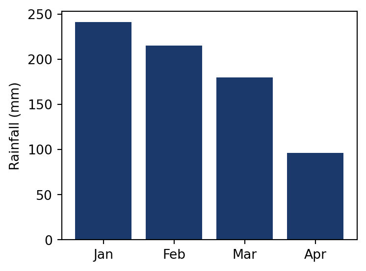
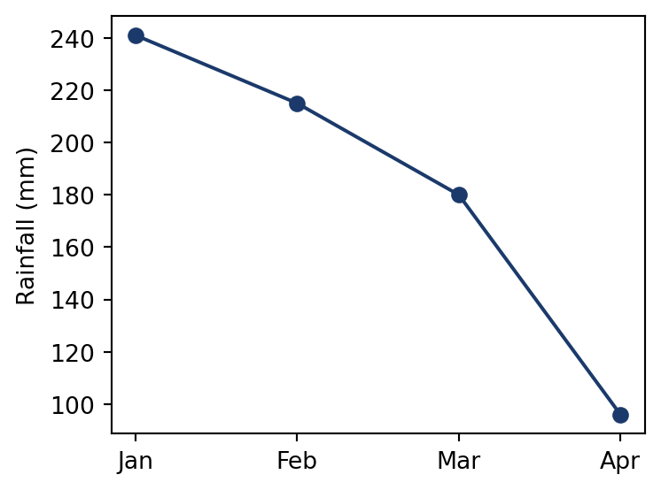
layout-ncol: 2 puts two plots side by side, and echo: false keeps the code out of the reader’s way:

```{python}
#| echo: false
#| layout-ncol: 2

plt.bar(rain["month"], rain["mm"])
plt.show()

plt.plot(rain["month"], rain["mm"])
plt.show()
```

What the reader sees:

Both figures came straight from the code at render time. Change the data and they update themselves

Engines: what actually runs your code

  • Quarto runs no code itself. It hands each chunk to an engine
  • Jupyter runs Python, and any language with a Jupyter kernel. knitr runs R
  • This course uses Jupyter. These slides render with jupyter: python3
  • Every render starts one fresh session and works through the chunks top to bottom
  • Chunks share state, like notebook cells: a variable from chunk one still exists in chunk ten
  • Fresh session, top to bottom. That is a restart-and-run-all test, every time
  • So a document that renders is one whose analysis just ran from scratch. Quarto checks your reproducibility for you
---
title: "My report"
format: html
jupyter: python3
---

Quarto can usually detect the engine from your chunks. Declaring it anyway tells the next reader what they need installed.

If you ever switch to R, change this one line and the rest of the document stays as it is

A minimal Python document

---
title: "Palmer Penguins Demo"
format:
  html:
    code-fold: true
jupyter: python3
---

## Meet Quarto

Quarto enables you to weave together content and
executable code into a finished document. To learn
more about Quarto see <https://quarto.org>.

```{python}
#| echo: false
#| message: false

import seaborn as sns
from palmerpenguins import load_penguins
sns.set_style('whitegrid')

penguins = load_penguins()

g = sns.lmplot(x="flipper_length_mm",
               y="body_mass_g",
               hue="species",
               height=7,
               data=penguins,
               palette=['#FF8C00','#159090','#A034F0'])
g.set_xlabels('Flipper Length')
g.set_ylabels('Body Mass')
  • Thirty lines, and everything from today’s lecture is in them
  • The YAML header names the document and picks the format and engine
  • code-fold: true tucks the code behind a toggle, so readers who want it can still find it
  • The prose is plain Markdown, with a ## heading
  • One chunk loads the penguin data and draws a figure
  • The next slide shows what renders

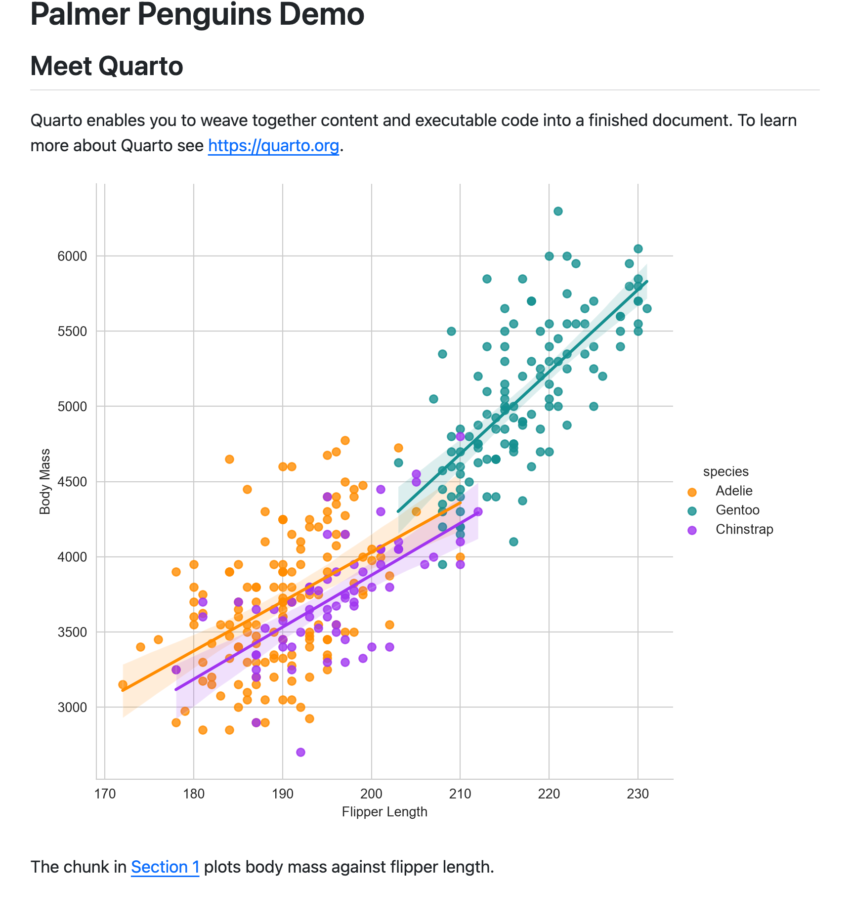
The rendered page

  • The title comes from the YAML, the heading and prose from the Markdown, and the figure from the chunk
  • The Code toggle at the top is code-fold: true at work
  • Change the data and render again: the figure and the numbers follow
  • This page cannot show a figure its own code did not produce. That is literate programming doing its job

Try it yourself!

Create a Quarto document from scratch and render it to HTML.

  1. Make a new file called weather.qmd
  2. Start it with this YAML header:
---
title: "Rainfall report"
author: "Your name"
format: html
jupyter: python3
---
  1. Add a ## heading and a short paragraph
  2. Add a chunk that builds the table below and prints it
  3. Add a second chunk that draws a bar chart, with its code hidden
  4. Render the file and open the result

Use this data so everyone gets the same answer:

import pandas as pd

rain = pd.DataFrame({
    "month": ["Jan", "Feb", "Mar", "Apr"],
    "mm": [241, 215, 180, 96]
})

Stuck? The option that hides code is on the chunk options slide, and quarto check diagnoses a broken installation

Answer: Appendix 01

Summary

  • The reproducibility crisis is real, and most computational results fail for a mundane reason: the code does not run
  • The ladder: re-runnable → reproducible → replicable → reusable. This course gets you to the second step
  • Four ingredients travel together: code, data, environment, documentation
  • The habits: raw data left untouched, cleaning in code, relative paths only, seeds set, versions written down, a README that says how to rebuild
  • Literate programming keeps text, code, and results in one file, so they cannot drift apart
  • Quarto is our tool for it: one plain-text .qmd file, one render command, many output formats

Next class

  • Quarto in practice: Markdown in depth, PDFs, and citations that format themselves
  • freeze: rendering documents without re-running the world
  • Slides (like these) and websites, published straight from GitHub
  • Parameterised reports: one file that writes a report for every country in your dataset
  • Bring a working Quarto installation: today’s exercise is the check 🤓

One source file, a report for every country. Next class you build this

Additional materials

And that’s all for today! 🥳

Thank you very much and see you soon! 😊 🙏🏼

Appendix 01: Solution to the exercise

The complete weather.qmd:

---
title: "Rainfall report"
author: "Your name"
format: html
jupyter: python3
---

## Rainfall in the first four months

Rainfall fell steadily from January to April, with April
receiving less than half of January's total.

```{python}
import pandas as pd

rain = pd.DataFrame({
    "month": ["Jan", "Feb", "Mar", "Apr"],
    "mm": [241, 215, 180, 96]
})

rain
```

```{python}
#| echo: false

import matplotlib.pyplot as plt

plt.bar(rain["month"], rain["mm"], color="#1B3A6B")
plt.ylabel("Rainfall (mm)")
plt.show()
```

Then render it:

Terminal
quarto render weather.qmd

#| echo: false is the option that hides the code but keeps the output, which is what question 5 asked for.

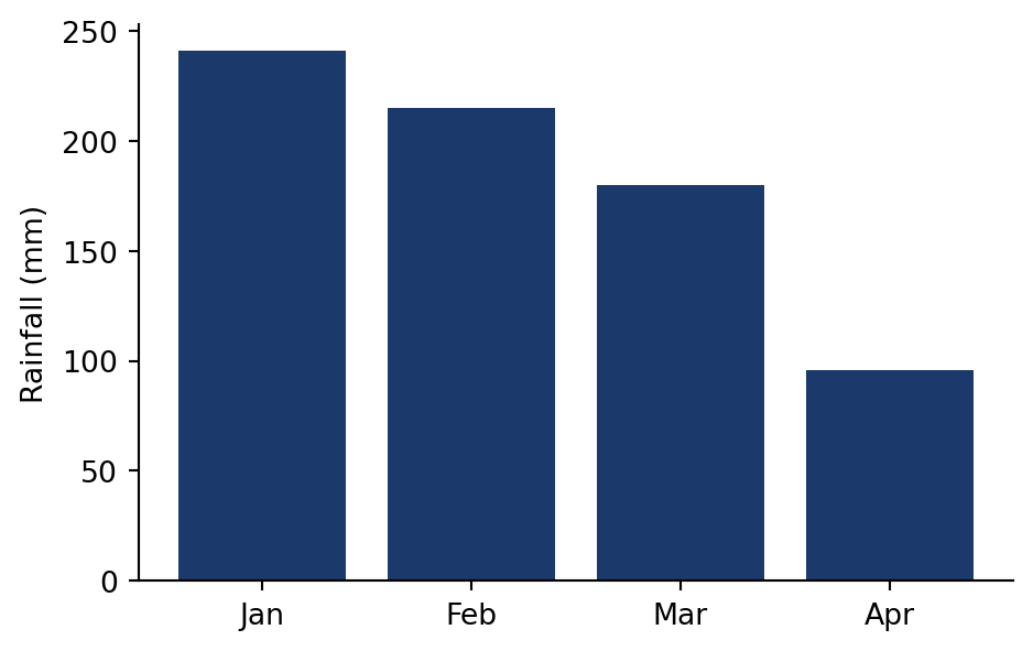
The chart your second chunk produces:

Back to the main text