library(kableExtra)
df <- mtcars[1:5, 1:6]
kable(df, "latex", booktabs = T) %>%
kable_styling(position = "center", font_size = 12) %>%
add_header_above(c(" " = 1, "Group 1" = 2, "Group 2" = 2,
"Group 3" = 1, "Group 4" = 1)) %>%
add_header_above(c(" ", "Group 5" = 4, "Group 6" = 2), bold = T) %>%
footnote(general = "Your comments go here.")Markdown Guide
How to Use This Guide
This guide is written in Markdown and uses the Quarto document format. Quarto is a powerful tool that allows you to write in Markdown and convert your document to a variety of formats, including PDF, HTML, and Word.
For you to use this template, you need to have R, Pandoc and Quarto installed on your computer. You can install Pandoc by following the instructions on the Pandoc website. To install the Quarto package, run the following command in R:
install.packages(c("quarto", "rmarkdown", "tidyverse"))You also need to install a distribution on your computer to convert your Markdown document to a PDF. I recommend you install TinyTeX, a lightweight distribution of . You can install TinyTeX by running the following command in R:
install.packages("tinytex")
tinytex::install_tinytex()
For those who prefer a more comprehensive distribution, you can install MiKTeX on Windows or MacTeX on macOS.
Finally, you should also install the Libertine and Inconsolata fonts on your computer to use this template. You can download the Libertine font from the Linux Libertine website and the Inconsolata font from the Google Fonts website. However, you can use any other font you prefer by changing the fontfamily and monofont options in the YAML header of this document. More information on how to change the font in your document can be found in the Quarto documentation.
You can then use the Quarto package to convert your Markdown document to a PDF. To convert your document to a PDF, run the following command in R:
quarto::quarto_render("pre-analysis-plan.qmd", output_format = "pdf")This command will convert your Markdown document to a PDF and save it in the same directory as your Markdown file.
How to Write Your Text Using Markdown
Markdown is a lightweight markup language that you can use to format your text. You can use Markdown to create headings, lists, tables, equations, and figures. Here are some examples of how to format your text using Markdown:
Headings
You can create headings using the # symbol. For example, # Heading 1 creates a first-level heading, ## Heading 2 creates a second-level heading, and so on. You can create up to six levels of headings using the # symbol.
Lists
To create an ordered list with nested unordered sub-items in Quarto, you can write the following code:
1. This is an ordered list.
2. This is the second item in the ordered list.
  - This is a sub-item in the unordered list.
- This is a sub-sub-item in the unordered list.- This is an ordered list.
- This is the second item in the ordered list.
- This is a sub-item in the unordered list.
- This is a sub-sub-item in the unordered list.
- This is a sub-item in the unordered list.
You can also create unordered lists:
- This is an unordered list.
- This is the second item in the unordered list.
- This is a sub-item in the unordered list.- This is an unordered list.
- This is the second item in the unordered list.
- This is a sub-item in the unordered list.
Tables
You can create tables using the | symbol. For example:
Table: Your Caption {#tbl-markdown}

| A            | New              | Table          |
|:-------------|:----------------:|---------------:|
|left-aligned  |centre-aligned    |right-aligned   |
|*italics* |~~strikethrough~~ |**boldface** || A | New | Table |
|---|---|---|
| left-aligned | centre-aligned | right-aligned |
| italics | boldface |
The : symbols in the second row of the table determine the alignment of the text in each column. You can use left, center, or right to align the text.
To use the kable and kableExtra packages in R for creating and customising tables, you first need to install these packages if you have not already. You can do this by running install.packages("knitr") and install.packages("kableExtra) in R. Below is an example. Please check the pre-analysis-plan.qmd file for the code.
This will create a table with the mtcars dataset from the datasets package in R. You can customise the table using the kableExtra package to add a caption, change the font size, and add headers above the columns. You can also add footnotes to the table using the footnote function.
Equations
You can create equations using the $$ symbol. For example in Equation 1, we have the formula for the standard deviation of a population:
$$
\sigma = \sqrt{\frac{\sum_{i=1}^{N} (x_i - \mu)^2}{N}}
$$ {#eq-stddev}
\[ \sigma = \sqrt{\frac{\sum_{i=1}^{N} (x_i - \mu)^2}{N}} \tag{1}\]
You can also create equations inline by using the $ symbol. For example, $\alpha = \beta + \gamma$ will render as \(\alpha = \beta + \gamma\). To learn more about how to write equations in using Markdown, you can refer to the Overleaf documentation.
Figures
You can include figures in your document using the {#fig-label} syntax. For example:
{#fig-label}This will include the image path/to/image.png in your document with the caption “This is a figure caption.” You can refer to the figure using the label fig-label.
You can also use the knitr package in R to create figures. This gives you more control over the appearance of the figure and allows you to include the code used to create the figure in your document. To include the same figure, you can use the following code:
library(knitr)
knitr::include_graphics("path/to/image.png")
There are many options you can use to customise the appearance of your figures, such as changing the width of the figure, adding a border, or changing the alignment. You can find more information on how to customise figures in the Quarto documentation.
Code Blocks and Syntax Highlighting
You can include code blocks in your document using triple backticks (```). For example, if you would like to include an R code block in your document, you can write ```{r}, and close it with another set of triple backticks (```). You can also add chunk options to the code block to control the output of the code block with #|. For example:
#| label: fig-airquality
#| fig-cap: "Temperature and ozone level."
#| warning: false

library(ggplot2)
ggplot(airquality, aes(Temp, Ozone)) +
  geom_point() +
  geom_smooth(method = "loess", se = FALSE)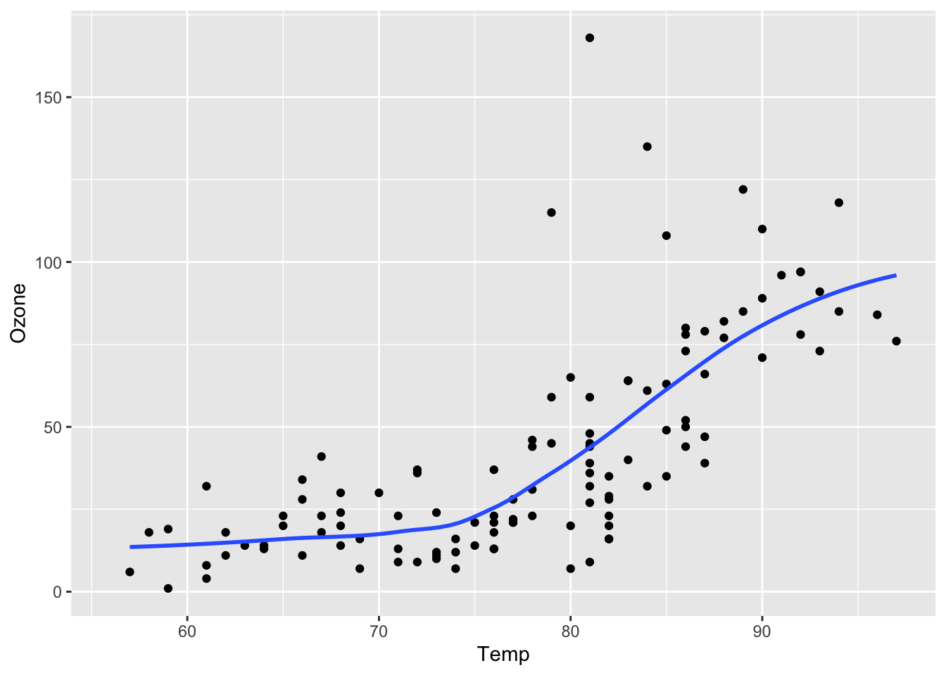
Quarto will run the code in the code block and include the output in the final document, as you can see in Figure 1. To learn more about code cell options, you can refer to the Quarto documentation.
Citations
You can include citations in your document using the @ symbol followed by the citation key. For example, @freire2018evaluating will create a citation to the reference with the key freire2018evaluating. You can also include page numbers in your citation by writing @freire2018evaluating [10--15]. The result will be: Freire (2018, 10–15). To include multiple citations in one bracket, you can write [@freire2018evaluating 10; @mignozzetti2022legislature 15]. This will create a citation like this: (Freire 2018, 10; Mignozzetti, Cepaluni, and Freire 2022, 15).
To include a bibliography in your document, you need to create a .bib file with your references and include it in the YAML header of your document. As you can find in the YAML header of this document:
bibliography: references.bibWhen searching for academic references, Google Scholar is an excellent tool for finding BibTeX citations. Here is a quick guide:
- Search for your desired reference on Google Scholar
- Look for the “Cite” button below the reference
- Click on “Cite” and then select “BibTeX” from the options
- Copy the generated BibTeX citation
- Paste it into your
.bibfile
This method makes it easy to maintain consistent and accurate citations in your academic work. Plus, it saves you the hassle of manually formatting each reference.
Footnotes
Quarto supports inline footnotes1. To create a footnote, simply add a caret and brackets with a label inside, like this: [^label]. Then, you can define the footnote content anywhere in the document using the same label followed by a colon2. I usually include them at the end of a paragraph. Quarto will automatically number and format your footnotes for you.
References
Freire, Danilo. 2018. “Evaluating the effect of homicide prevention strategies in São Paulo, Brazil: A synthetic control approach.” Latin American Research Review 53 (2): 231–49.
Mignozzetti, Umberto, Gabriel Cepaluni, and Danilo Freire. 2022. “Legislature Size and Welfare: Evidence from Brazil.” American Journal of Political Science, 1–17.