class: center, middle, inverse, title-slide # Week 13 - Uncertainty ## Review <html> <div style="float:left"> </div> <hr color='#EB811B' size=1px width=800px> </html> ### Danilo Freire ### 26 April 2019 --- <style> .remark-slide-number { position: inherit; } .remark-slide-number .progress-bar-container { position: absolute; bottom: 0; height: 6px; display: block; left: 0; right: 0; } .remark-slide-number .progress-bar { height: 100%; background-color: #EB811B; } .orange { color: #EB811B; } </style> # Today's Agenda .font150[ * Questions about final project * Review: - Uncertainty - Standard errors - Confidence intervals - Hypothesis testing - Ordinary least squares regression - P-values - (Robust) Standard errors ] --- class: inverse, center, middle # How is the project going? <html><div style='float:left'></div><hr color='#EB811B' size=1px width=720px></html> --- # Review: Uncertainty .font150[ * It is usually unfeasible to analyse the entire population * So if we want to test a hypothesis, we can rarely know for sure what is the value of the population .orange[parameter] `\(\theta\)` - How many Americans support Donald Trump? - If we give cash to all poor Argentinians, would their health improve? - How what is the effect of a new blood pressure medicine in all adult males? * We must take a sample of the population of interest and estimate some quantity of interest `\(\hat{\theta}\)` ] --- # Review: Uncertainty .font150[ * Goal of inferential statistics: .orange[accurate and precise estimates] - Accurate: not very far from the true quantity of interest - Precise: with low levels of uncertainty * In an ideal world, we should have no estimation error: `\(\hat{\theta} = \theta\)` * But we often only have _one sample_ from our population * We have to be clear about how .orange[uncertain] our estimates are ] --- # Review: Standard Errors .font150[ * The way we convey uncertainty in statistics is with .orange[standard errors] * .orange[Standard error] is the _theoretical standard deviation_ of the population distribution * But we do not have access to that distribution * So we _assume_ the distribution is normal and use what we know about it * We know that, from the mean, plus or minus 2 standard deviations cover 95% of the area of the normal distribution ] --- # Review: Confidence Intervals .font150[ * .orange[Confidence intervals] are a range of potential values of the unknown population parameter * Since we do not know the true parameter value, we have to accept it might be anywhere in a given interval * By convention, we use _2 standard errors from the model coefficient_ (both to the right and left) as our confidence interval * It means we assume our model estimate is true, then we add uncertainty to it ] --- # Review: Confidence Intervals .font150[ * Remember: confidence intervals _do not_ represent 95% chance that the interval contains the true value * It means that, should we repeat the same experiment again and again, 95% of the time the confidence interval would contain the true population value * But unfortunately we often just have _one_ experiment * So, again, we assume our experiment is in the 95% that contains the true value * Meta-analysis: collect many studies and test them together ] --- # Review: Hypothesis Testing .font140[ * Often are interested if one variable `\(X\)` has an effect on another variable `\(Y\)` - Does capitalism cause democratisation? - Does oil make a country more corrupt? - Does foreign aid foster economic growth? * So we set up two hypotheses: - `\(X\)` does not have an effect on `\(Y = H_0\)` - `\(X\)` does not have an effect on `\(Y = H_1\)` * How are they called?] -- .font150[ * .orange[Null and alternative hypotheses] ] --- # Review: P-Value .font150[ * .orange[P-value] is the chance that, if `\(H_0\)` is true, we would observe a result like, or rarer than, the result we have at hand * By convention, we use `\(p < 0.05\)` - If there is less than 5% probability we could observe a given result if there was no effect of `\(X\)` on `\(Y\)`, we assume it is not by chance alone * If `\(p < 0.05\)`, we say the result is _statistically significant_ * .orange[Statistical significance does not imply practical significance] ] --- class: clear .center[] --- class: clear .center[] --- class: clear .center[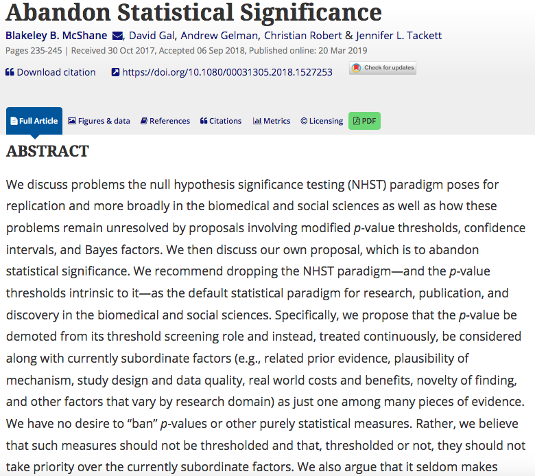] --- # Review: OLS and lm() .font150[ * _But while we do not abandon p-values_... ] -- .font150[ * ... we still have to learn how to read and use them * `summary(model <- lm(Y ~ X, data = dataset))` shows the coefficients, standard errors and associated p-values ] --- # OLS Example .font100[ ```r library(Zelig) # simulated data data(voteincome) summary(lm(income ~ education + age + female, data = voteincome)) ``` ``` ## ## Call: ## lm(formula = income ~ education + age + female, data = voteincome) ## ## Residuals: ## Min 1Q Median 3Q Max ## -10.2375 -2.0897 0.4316 2.1580 7.9853 ## ## Coefficients: ## Estimate Std. Error t value Pr(>|t|) ## (Intercept) 8.733125 0.397641 21.962 < 2e-16 *** ## education 1.956612 0.085341 22.927 < 2e-16 *** ## age -0.023194 0.004977 -4.660 3.44e-06 *** ## female -0.561721 0.170102 -3.302 0.000982 *** ## --- ## Signif. codes: 0 '***' 0.001 '**' 0.01 '*' 0.05 '.' 0.1 ' ' 1 ## ## Residual standard error: 3.264 on 1496 degrees of freedom ## Multiple R-squared: 0.3066, Adjusted R-squared: 0.3052 ## F-statistic: 220.5 on 3 and 1496 DF, p-value: < 2.2e-16 ``` ] --- # Review: OLS Assumptions .font150[ * For our coefficients to be unbiased, the linear model has to meet two assumptions: - .orange[Exogeneity:] no omitted variable that correlates with independent variables (parents' iq and books, academic achievement) - .orange[Homoscedasticity:] data points should be evenly distributed along the regression line * How to fix the first? And the second? ] -- .font150[ * First: .orange[randomisation]. Why? * Second: .orange[robust standard errors] ] --- # Review: Robust Standard Errors .font150[ * Fixes the problem of .orange[heteroscedasticity] - Distance from points to line (variance) is not constant * Easy to implement: - `sandwich` - `estimatr` * If you're running a linear model, when should you use them? ] -- .font150[ * .orange[_Always!_] ] --- # Review: lm_robust() .font150[ ```r mortality <- read.csv("https://raw.githubusercontent.com/pols1600/pols1600.github.io/master/datasets/prediction/bivariate_data.csv") library(estimatr) ``` ] --- # Review: lm_robust() .font110[ ```r m1 <- lm_robust(Child.Mortality ~ log(GDP) + PolityIV, mortality) summary(m1) ``` ``` ## ## Call: ## lm_robust(formula = Child.Mortality ~ log(GDP) + PolityIV, data = mortality) ## ## Standard error type: HC2 ## ## Coefficients: ## Estimate Std. Error t value Pr(>|t|) CI Lower CI Upper DF ## (Intercept) 424.339 5.07487 83.62 0.000e+00 414.390 434.287 6187 ## log(GDP) -39.922 0.56688 -70.42 0.000e+00 -41.033 -38.811 6187 ## PolityIV -2.307 0.08902 -25.91 1.274e-140 -2.481 -2.132 6187 ## ## Multiple R-squared: 0.615 , Adjusted R-squared: 0.6148 ## F-statistic: 4335 on 2 and 6187 DF, p-value: < 2.2e-16 ``` ] --- # Review: Clustered Robust SEs .font150[ * Social science data are often organised in clusters: - Average SAT scores for 5 schools from 2000 to 2010 - Gini index for 100 countries from 1945 to 2010 - Daily blood pressure measuments for 1,000 people for 2 months * _Some observations are clearly correlated with each other_: Gini index in Argentina in 1970 is correlated with the measure in 1971 * Our standard errors are biased because of that: clusters are not evenly distributed ] --- # Review: Clustered Robust SEs .font150[ ```r # Downlad Fearon and Laitin (2003) data temp <- tempfile() # create temporary file download.file("https://web.stanford.edu/group/ethnic/publicdata/repdata.zip", temp) library(haven) # read Stata .dta civilwars <- read_dta(unz(temp, "repdata.dta")) unlink(temp) ``` ] --- # Review: Clustered Robust SEs .font150[ ```r head(civilwars[,c(5,2,20)], 10) ``` ``` ## # A tibble: 10 x 3 ## year country gdpen ## <dbl> <chr> <dbl> ## 1 1945 USA 7.63 ## 2 1946 USA 7.65 ## 3 1947 USA 8.02 ## 4 1948 USA 8.27 ## 5 1949 USA 8.04 ## 6 1950 USA 8.77 ## 7 1951 USA 9.11 ## 8 1952 USA 9.07 ## 9 1953 USA 9.30 ## 10 1954 USA 9.09 ``` ] --- # Review: Clustered Robust SEs .font110[ ```r # add clusters = Country.code m1 <- lm_robust(Child.Mortality ~ log(GDP) + PolityIV, clusters = Country.code, data = mortality) summary(m1) ``` ``` ## ## Call: ## lm_robust(formula = Child.Mortality ~ log(GDP) + PolityIV, data = mortality, ## clusters = Country.code) ## ## Standard error type: CR2 ## ## Coefficients: ## Estimate Std. Error t value Pr(>|t|) CI Lower CI Upper DF ## (Intercept) 424.339 22.2811 19.045 1.784e-26 379.73 468.950 57.36 ## log(GDP) -39.922 2.4400 -16.361 2.780e-22 -44.82 -35.027 52.60 ## PolityIV -2.307 0.3382 -6.821 1.885e-09 -2.98 -1.633 76.18 ## ## Multiple R-squared: 0.615 , Adjusted R-squared: 0.6148 ## F-statistic: 191.9 on 2 and 153 DF, p-value: < 2.2e-16 ``` ] --- class: clear .center[] .font150[ <https://doi.org/10.1038/s41562-019-0572-z> ] --- class: clear .center[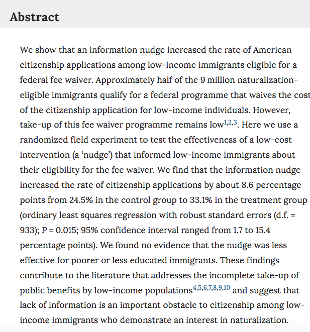] --- class: clear .center[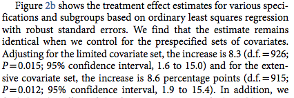] --- class: clear .center[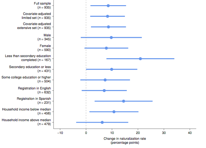] --- class: inverse, center, middle # Questions? <html><div style='float:left'></div><hr color='#EB811B' size=1px width=720px></html> --- class: inverse, center, middle # See you next week! <html><div style='float:left'></div><hr color='#EB811B' size=1px width=720px></html>