Week 13 - Uncertainty

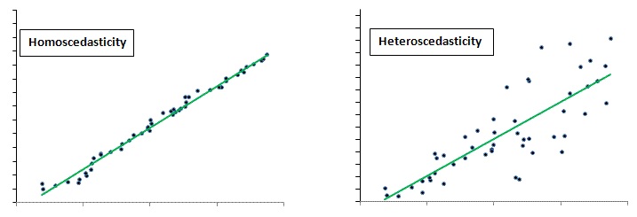
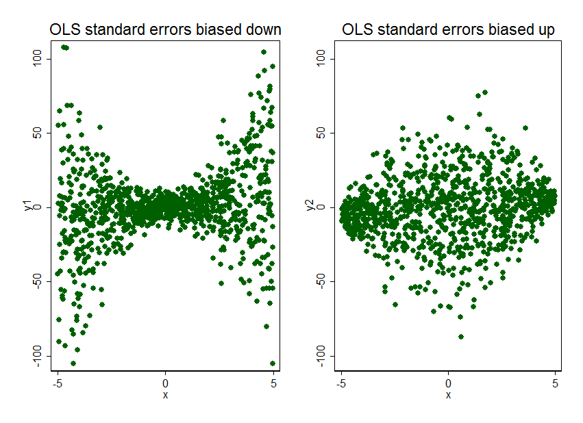
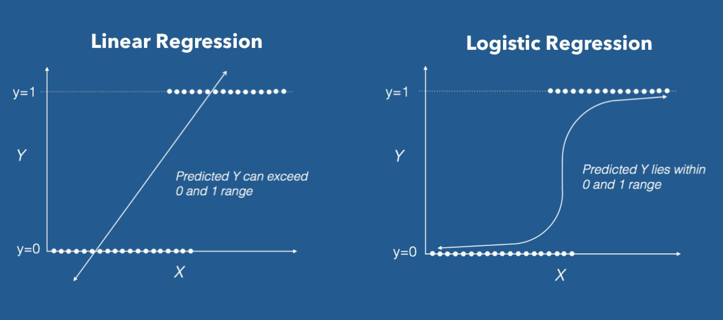
# Week 13 - Uncertainty
## OLS Assumptions, Robust Standard Errors, Logit
<html>
<div style="float:left">

</div>
<hr color='#EB811B' size=1px width=800px>
</html>
### Danilo Freire
### 24 April 2019

---

<style>

.remark-slide-number {
  position: inherit;
}

.remark-slide-number .progress-bar-container {
  position: absolute;
  bottom: 0;
  height: 6px;
  display: block;
  left: 0;
  right: 0;
}

.remark-slide-number .progress-bar {
  height: 100%;
  background-color: #EB811B;
}

.orange {
  color: #EB811B;
}
</style>

# Today's Agenda

* Assumptions: exogeneity and homoscedasticity

* Robust standard errors

* `estimatr` package

* Logistic regression
]
---

# Model Assumptions

# Model Assumptions

---

# Regression with Uncertainty

* where `$\mathbb{E}(\epsilon_i) = 0$` and `$\mathbb{V}(\epsilon_i)=\sigma^2$`

* Estimation of parameters via .orange[least squares:]

`$$\textsf{minimize SSR} \quad \textsf{where} \quad \textsf{SSR} \ = \ \sum_{i=1}^n \hat\epsilon_i^2 \ =$$` `$$\sum_{i=1}^n (y_i - \hat\beta_0 - \hat\beta_1 x_i)^2$$`
]
---

# Exogeneity and Homoskedasticity

- .orange[Exogeneity:] the mean of `$\epsilon_i$` does not depend on `$x_i$` 
      `$$\mathbb{E}(\epsilon_i \mid x_i) \ = \ \mathbb{E}(\epsilon_i) \ = \ 0$$`
      
  - .orange[Homoscedasticity:] the variance of `$\epsilon_i$` does not
      depend on `$x_i$`
      `$$\mathbb{V}(\epsilon_i \mid x_i) \ = \ \mathbb{V}(\epsilon_i) \ = \ \sigma^2$$`
]
--
.font150[
* When is each assumption violated?

* What to do in those cases?
]
---

# Exogeneity

.font150[
* Exogeneity means that the unobserved causes of the dependent variable are _uncorrelated_ with the variables we include in our model

* This is a _very strong assumption_ in observational studies

* Why? Because of _omitted variable bias_

* .orange[Omitted variable bias:] when there is another factor that causes the independent variables, but we didn't include them in our model
  - We didn't think of it
  - Hard to measure
]

---

# Omitted Variable Bias

* If an important variable is missing, the coefficients will be incorrect

* The independent variables we have can either become statistically significant or not, negative or positive, we cannot know for sure

* Difficult to verify in observational studies
]
---

# Omitted Variable Bias

# Omitted Variable Bias

# Omitted Variable Bias

# Omitted Variable Bias

# Exogeneity

* Very little in terms of statistical analysis

* The best solution is to run _a randomised experiment_, whenever feasible

* Why?
]
--
.font150[
* If the treatment is allocated at random we know it is not correlated with _anything_

* So there is lower risk of omitted variable bias
]
---

# Homoscedasticity

.font150[
* Homoscedasticity means that the value of standard errors are constant along all values of our independent variables

* _This is often not the case either_

* But there is an easy statistical fix for the problem: .orange[robust standard errors]

* Robust standard errors are usually (but not always) larger than regular standard errors

* So they are _more conservative_: it is more difficult for a result to be statistically significant
]
---

# Homoscedasticity

# Homoscedasticity

# Robust Standard Errors

* `R` has many packages that compute robust standard errors

* New, easy to use package: `estimatr`

* `lm_robust(Y ~  X, data = your_data)`
]
---

# Robust Standard Errors

```r
mortality <- read.csv("https://raw.githubusercontent.com/pols1600/pols1600.github.io/master/datasets/prediction/bivariate_data.csv")
summary(lm(Child.Mortality ~ log(GDP) + PolityIV, mortality))
```

```
## 
## Call:
## lm(formula = Child.Mortality ~ log(GDP) + PolityIV, data = mortality)
## 
## Residuals:
##      Min       1Q   Median       3Q      Max 
## -142.891  -30.449   -3.328   21.529  212.403 
## 
## Coefficients:
##              Estimate Std. Error t value Pr(>|t|)    
## (Intercept) 424.33897    4.45762   95.19   <2e-16 ***
## log(GDP)    -39.92202    0.51740  -77.16   <2e-16 ***
## PolityIV     -2.30666    0.08396  -27.47   <2e-16 ***
## ---
## Signif. codes:  0 '***' 0.001 '**' 0.01 '*' 0.05 '.' 0.1 ' ' 1
## 
## Residual standard error: 46.55 on 6187 degrees of freedom
##   (24422 observations deleted due to missingness)
## Multiple R-squared:  0.615,	Adjusted R-squared:  0.6148 
## F-statistic:  4941 on 2 and 6187 DF,  p-value: < 2.2e-16
```
]
---

# Robust Standard Errors

```r
library(estimatr)
summary(lm_robust(Child.Mortality ~ log(GDP) + PolityIV, mortality))
```

```
## 
## Call:
## lm_robust(formula = Child.Mortality ~ log(GDP) + PolityIV, data = mortality)
## 
## Standard error type:  HC2 
## 
## Coefficients:
##             Estimate Std. Error t value   Pr(>|t|) CI Lower CI Upper   DF
## (Intercept)  424.339    5.07487   83.62  0.000e+00  414.390  434.287 6187
## log(GDP)     -39.922    0.56688  -70.42  0.000e+00  -41.033  -38.811 6187
## PolityIV      -2.307    0.08902  -25.91 1.274e-140   -2.481   -2.132 6187
## 
## Multiple R-squared:  0.615 ,	Adjusted R-squared:  0.6148 
## F-statistic:  4335 on 2 and 6187 DF,  p-value: < 2.2e-16
```
]
---

# Clustered Standard Errors

* They account for heteroskedasticity across "clusters" of observations (such as states, schools, or individuals)

* Used when the data consist of repeated observations of the same units over time
    - E.g.: 10 countries from 1970 to 1980

* Clustered standard errors are also easily estimated with `estimatr`
]
---

# Clustered Standard Errors

```r
library(estimatr)
summary(lm_robust(Child.Mortality ~ log(GDP) + PolityIV, clusters = Country.code, mortality))
```

```
## 
## Call:
## lm_robust(formula = Child.Mortality ~ log(GDP) + PolityIV, data = mortality, 
##     clusters = Country.code)
## 
## Standard error type:  CR2 
## 
## Coefficients:
##             Estimate Std. Error t value  Pr(>|t|) CI Lower CI Upper    DF
## (Intercept)  424.339    22.2811  19.045 1.784e-26   379.73  468.950 57.36
## log(GDP)     -39.922     2.4400 -16.361 2.780e-22   -44.82  -35.027 52.60
## PolityIV      -2.307     0.3382  -6.821 1.885e-09    -2.98   -1.633 76.18
## 
## Multiple R-squared:  0.615 ,	Adjusted R-squared:  0.6148 
## F-statistic: 191.9 on 2 and 153 DF,  p-value: < 2.2e-16
```
]
---

# Suggestions

* They correct for heteroscedasticity when necessary, but do nothing when standard errors are homoscedastic

* .orange[They do not change the value of the coefficients], so your effect size is the same

* No need to do any additional calculations, just use the `lm_robust()` function from `estimatr`

* If you have panel data (repeated observations from the same units over time), use clustered standard errors
]
---

# Logistic Regression

* E.g.: vote (yes or no), pass/fail, win/lose, alive/dead, healthy/sick

* It is possible to estimate a linear model with a binary dependent variable

* However, it is very likely that the homoscedasticity assumption is violated

* Two solutions:
    - Robust/Clustered standard errors
    - _Logistic regression_
]
---

# Logistic Regression

.font150[
* Logistic regression transforms the linear model so that the values are restricted to 0 or 1

* Linear model: `$Y = \beta_0 + \beta_1 x_1 + ...+ \epsilon$`

* Logistic regression: `$Y = \frac{1}{1 + exp^{- (\beta_0 + \beta_1 x_1 + ...+ \epsilon)}}$`

* Good for modelling probabilities

* In R: `glm(Y ~ X1 + X2, binomial("logit"), yourdata)`

* Somewhat tricky to interpret
]
---

# Logistic Regression

---

# Logistic Regression

```r
# download and open a zipped .dta file from a URL

temp <- tempfile() # create temporary file
download.file("https://web.stanford.edu/group/ethnic/publicdata/repdata.zip", temp)

library(haven) # read Stata .dta

civilwars <- read_dta(unz(temp, "repdata.dta")) # load dta
unlink(temp) # delete temporary file

names(civilwars)
```

```
##  [1] "ccode"      "country"    "cname"      "cmark"      "year"      
##  [6] "wars"       "war"        "warl"       "onset"      "ethonset"  
## [11] "durest"     "aim"        "casename"   "ended"      "ethwar"    
## [16] "waryrs"     "pop"        "lpop"       "polity2"    "gdpen"     
## [21] "gdptype"    "gdpenl"     "lgdpenl1"   "lpopl1"     "region"    
## [26] "western"    "eeurop"     "lamerica"   "ssafrica"   "asia"      
## [31] "nafrme"     "colbrit"    "colfra"     "mtnest"     "lmtnest"   
## [36] "elevdiff"   "Oil"        "ncontig"    "ethfrac"    "ef"        
## [41] "plural"     "second"     "numlang"    "relfrac"    "plurrel"   
## [46] "minrelpc"   "muslim"     "nwstate"    "polity2l"   "instab"    
## [51] "anocl"      "deml"       "empethfrac" "empwarl"    "emponset"  
## [56] "empgdpenl"  "emplpopl"   "emplmtnest" "empncontig" "empolity2l"
## [61] "sdwars"     "sdonset"    "colwars"    "colonset"   "cowwars"   
## [66] "cowonset"   "cowwarl"    "sdwarl"     "colwarl"
```
]
---

# Logistic Regression

```r
civilwars$ethonset <- ifelse(civilwars$ethonset >= 1, 1, civilwars$ethonset)
summary(glm(ethonset ~ lgdpenl1 + polity2l, binomial("logit"), civilwars))
```

```
## 
## Call:
## glm(formula = ethonset ~ lgdpenl1 + polity2l, family = binomial("logit"), 
##     data = civilwars)
## 
## Deviance Residuals: 
##     Min       1Q   Median       3Q      Max  
## -0.5119  -0.1734  -0.1337  -0.0992   3.3698  
## 
## Coefficients:
##             Estimate Std. Error z value Pr(>|z|)    
## (Intercept)  1.17383    0.93400   1.257    0.209    
## lgdpenl1    -0.76896    0.13131  -5.856 4.74e-09 ***
## polity2l     0.02720    0.01917   1.419    0.156    
## ---
## Signif. codes:  0 '***' 0.001 '**' 0.01 '*' 0.05 '.' 0.1 ' ' 1
## 
## (Dispersion parameter for binomial family taken to be 1)
## 
##     Null deviance: 787.71  on 6326  degrees of freedom
## Residual deviance: 750.95  on 6324  degrees of freedom
##   (283 observations deleted due to missingness)
## AIC: 756.95
## 
## Number of Fisher Scoring iterations: 8
```
]
---

# Linear model - Robust SEs

```r
summary(lm_robust(ethonset ~ lgdpenl1 + polity2l, civilwars))
```

```
## 
## Call:
## lm_robust(formula = ethonset ~ lgdpenl1 + polity2l, data = civilwars)
## 
## Standard error type:  HC2 
## 
## Coefficients:
##               Estimate Std. Error t value  Pr(>|t|)   CI Lower   CI Upper
## (Intercept)  0.0754590  0.0134397   5.615 2.053e-08  4.911e-02  0.1018053
## lgdpenl1    -0.0083556  0.0016424  -5.087 3.735e-07 -1.158e-02 -0.0051359
## polity2l     0.0003086  0.0001861   1.658 9.735e-02 -5.625e-05  0.0006734
##               DF
## (Intercept) 6324
## lgdpenl1    6324
## polity2l    6324
## 
## Multiple R-squared:  0.005672 ,	Adjusted R-squared:  0.005358 
## F-statistic: 14.86 on 2 and 6324 DF,  p-value: 3.656e-07
```
]
---

# Linear model - Clustered SEs

```r
summary(lm_robust(ethonset ~ lgdpenl1 + polity2l, cluster = country, civilwars))
```

```
## 
## Call:
## lm_robust(formula = ethonset ~ lgdpenl1 + polity2l, data = civilwars, 
##     clusters = country)
## 
## Standard error type:  CR2 
## 
## Coefficients:
##               Estimate Std. Error t value  Pr(>|t|)   CI Lower   CI Upper
## (Intercept)  0.0754590  0.0173372   4.352 4.626e-05  4.086e-02  0.1100535
## lgdpenl1    -0.0083556  0.0020983  -3.982 1.725e-04 -1.254e-02 -0.0041664
## polity2l     0.0003086  0.0001881   1.640 1.045e-01 -6.526e-05  0.0006824
##                DF
## (Intercept) 68.14
## lgdpenl1    66.17
## polity2l    89.02
## 
## Multiple R-squared:  0.005672 ,	Adjusted R-squared:  0.005358 
## F-statistic:  8.35 on 2 and 155 DF,  p-value: 0.0003597
```
]
---

# Logistic or Linear Regression?

.font150[
* If you run a linear model with robust standard errors, the results are similar to those from the logistic regression

* Varies according to the discipline: 
    - In statistics and political science, researchers prefer logistic regressions
    - In economics, they use linear models
    
* If you're writing an article, use both and check if your results are consistent
]

---

# Questions?

<html><div style='float:left'></div><hr color='#EB811B' size=1px width=720px></html>  
---

# See you on Friday!