class: center, middle, inverse, title-slide # Week 12 - Uncertainty ## Standard Errors and P-Values <html> <div style="float:left"> </div> <hr color='#EB811B' size=1px width=800px> </html> ### Danilo Freire ### 17 April 2019 --- <style> .remark-slide-number { position: inherit; } .remark-slide-number .progress-bar-container { position: absolute; bottom: 0; height: 6px; display: block; left: 0; right: 0; } .remark-slide-number .progress-bar { height: 100%; background-color: #EB811B; } .orange { color: #EB811B; } </style> # Confidence Intervals .font130[ * `\(\alpha\)` is the probability of rejecting the null hypothesis when it is in fact true * Select a value for `\(\alpha\)`, usually 0.05. * So we expect every 1 in 20 (5/100) confidence intervals to be false if we use `\(\alpha = 0.05\)` * Then, we select the _critical value_: `\(z = 1 - \alpha\)`. This is a point of the test distribution (usually the normal) that determines whether to reject the null hypothesis * `\(z\)` is the number of standard deviations of the distribution * We usually use 1.96, often rounded to 2 ] --- # Confidence Intervals .font150[ * The confidence interval you will see most often is this one: `$$CI(\alpha) = \overline{X} - 1.96 \times SE, \overline{X} + 1.96 \times SE$$` * Why? Beause if you take the mean of the normal distribution and add `\(\pm 2 \times SE\)` you will cover 95% of the area * .orange[When evaluating effects, we usually judge them based on whether the 95% confidence interval covers zero or not] * If it covers zero, there is a possibility that the effect is, well, zero. Zero effect = no relationship between variables ] --- # Average Treatment Effects .font150[ * How do we estimate the ATE in RTCs? * Difference in means between treatment and control group * Sample average in treated group `\(\overline{X}_{t}\)` and control group `\(\overline{X}_{c}\)` * SE treated: `\(\hat{SE}_{t} = \sqrt{\frac{\hat{\sigma}^{2}_{t}}{N_{t}}}\)` * SE control: `\(\hat{SE}_{c} = \sqrt{\frac{\hat{\sigma}^{2}_{c}}{N_{c}}}\)` * What do we use for `\(\sigma^2\)`? The variance of the sample, as we don't have the variance of the full sampling distribution ] --- # Average Treatment Effects .font150[ * We can use these SEs to construct confidence intervals around each of the averages * But we need to construct SEs _around the difference in means itself_ `\((\overline{X}_{t} - \overline{X}_{c})\)` * `\(\hat{SE}_{t-c} = \sqrt{\frac{\mathbb{V}(X_{t})}{N_{t}} + \frac{\mathbb{V}(X_{c})}{N_{c}}}\)` ] --- # Average Treatment Effects .font140[ * We can use the standard error to construct a 95% confidence interval for the difference in means: * Example: ATE = 3.5, SE = 2.65 * What is the confidence interval? ] -- .font140[ * `\(CI(0.05) = 3.5 - 1.96 \times 2.65 = -1,694\)` * `\(CI(0.05) = 3.5 + 1.96 \times 2.65 = 8.694\)` * Is the difference statistically significant? ] -- .font140[ * _No_, as the difference between the treatment and control groups can be zero ] --- # The summary function in R .font150[ * R has a convenient function to see if the results are statistically significant * `summary(name_of_your_model)` * It shows the coefficient, the standard error, and the significance level all at once ] --- # Example 1 - Resume ```r resume <- read.csv("https://raw.githubusercontent.com/pols1600/pols1600.github.io/master/datasets/causality/resume.csv") model1 <- lm(call ~ race, data = resume) summary(model1) ``` ``` ## ## Call: ## lm(formula = call ~ race, data = resume) ## ## Residuals: ## Min 1Q Median 3Q Max ## -0.09651 -0.09651 -0.06448 -0.06448 0.93552 ## ## Coefficients: ## Estimate Std. Error t value Pr(>|t|) ## (Intercept) 0.064476 0.005505 11.713 < 2e-16 *** ## racewhite 0.032033 0.007785 4.115 3.94e-05 *** ## --- ## Signif. codes: 0 '***' 0.001 '**' 0.01 '*' 0.05 '.' 0.1 ' ' 1 ## ## Residual standard error: 0.2716 on 4868 degrees of freedom ## Multiple R-squared: 0.003466, Adjusted R-squared: 0.003261 ## F-statistic: 16.93 on 1 and 4868 DF, p-value: 3.941e-05 ``` --- # Example 1 - Resume ```r resume <- read.csv("https://raw.githubusercontent.com/pols1600/pols1600.github.io/master/datasets/causality/resume.csv") model2 <- lm(call ~ sex, data = resume) summary(model2) ``` ``` ## ## Call: ## lm(formula = call ~ sex, data = resume) ## ## Residuals: ## Min 1Q Median 3Q Max ## -0.08249 -0.08249 -0.08249 -0.07384 0.92616 ## ## Coefficients: ## Estimate Std. Error t value Pr(>|t|) ## (Intercept) 0.082488 0.004446 18.555 <2e-16 *** ## sexmale -0.008645 0.009253 -0.934 0.35 ## --- ## Signif. codes: 0 '***' 0.001 '**' 0.01 '*' 0.05 '.' 0.1 ' ' 1 ## ## Residual standard error: 0.2721 on 4868 degrees of freedom ## Multiple R-squared: 0.0001792, Adjusted R-squared: -2.614e-05 ## F-statistic: 0.8727 on 1 and 4868 DF, p-value: 0.3502 ``` --- # Example 1 - Resume ```r resume <- read.csv("https://raw.githubusercontent.com/pols1600/pols1600.github.io/master/datasets/causality/resume.csv") model3 <- lm(call ~ race + sex, data = resume) summary(model3) ``` ``` ## ## Call: ## lm(formula = call ~ race + sex, data = resume) ## ## Residuals: ## Min 1Q Median 3Q Max ## -0.09866 -0.09866 -0.06653 -0.06653 0.94259 ## ## Coefficients: ## Estimate Std. Error t value Pr(>|t|) ## (Intercept) 0.066534 0.005886 11.304 < 2e-16 *** ## racewhite 0.032130 0.007786 4.127 3.74e-05 *** ## sexmale -0.009128 0.009239 -0.988 0.323 ## --- ## Signif. codes: 0 '***' 0.001 '**' 0.01 '*' 0.05 '.' 0.1 ' ' 1 ## ## Residual standard error: 0.2716 on 4867 degrees of freedom ## Multiple R-squared: 0.003666, Adjusted R-squared: 0.003256 ## F-statistic: 8.953 on 2 and 4867 DF, p-value: 0.0001314 ``` --- # Example 2 - Child Mortality ```r mortality <- read.csv("https://raw.githubusercontent.com/pols1600/pols1600.github.io/master/datasets/prediction/bivariate_data.csv") summary(lm(Child.Mortality ~ log(GDP) + PolityIV, data = mortality)) ``` ``` ## ## Call: ## lm(formula = Child.Mortality ~ log(GDP) + PolityIV, data = mortality) ## ## Residuals: ## Min 1Q Median 3Q Max ## -142.891 -30.449 -3.328 21.529 212.403 ## ## Coefficients: ## Estimate Std. Error t value Pr(>|t|) ## (Intercept) 424.33897 4.45762 95.19 <2e-16 *** ## log(GDP) -39.92202 0.51740 -77.16 <2e-16 *** ## PolityIV -2.30666 0.08396 -27.47 <2e-16 *** ## --- ## Signif. codes: 0 '***' 0.001 '**' 0.01 '*' 0.05 '.' 0.1 ' ' 1 ## ## Residual standard error: 46.55 on 6187 degrees of freedom ## (24422 observations deleted due to missingness) ## Multiple R-squared: 0.615, Adjusted R-squared: 0.6148 ## F-statistic: 4941 on 2 and 6187 DF, p-value: < 2.2e-16 ``` --- # Confidence Intervals .font150[ * To recap: * When you're reading articles or writing your own, there's an easy way to see if the effect is statistically significant with `\(pvalue < 0.05\)` * Only three steps: - Check the model coefficient - Check the standard error and multiply it by two - Sum and subtract the value from the coefficient. If it gives you zero, it's not significant. If it doesn't include zero, it is statistically significant ] --- # Example 3 - Civil Wars .center[] --- # Example 3 - Civil Wars .center[] --- # Example 4 - Nurses .center[] --- # Example 4 - Nurses .center[] --- # Linear Models .font150[ * Next week, we will discuss in further details the statistical assumptions behind the linear model ] --- # Statistical Significance Controversy .center[] .font150[ <https://www.nature.com/articles/d41586-019-00857-9> ] --- # Statistical Significance Controversy .center[] --- # Statistical Significance Controversy .center[] --- # Statistical Significance Controversy .center[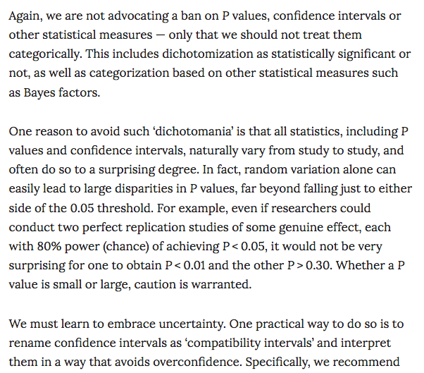] --- class: inverse, center, middle # Questions? <html><div style='float:left'></div><hr color='#EB811B' size=1px width=720px></html> --- class: inverse, center, middle # See you next week! <html><div style='float:left'></div><hr color='#EB811B' size=1px width=720px></html>