Week 08 - Regression

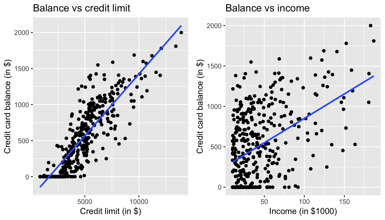
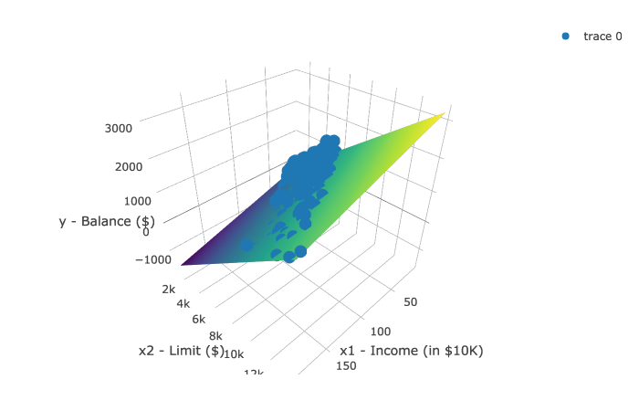
# Week 08 - Regression
## Multivariate Models, Statistical Control and Standardised Coefficients
<html>
<div style="float:left">

</div>
<hr color='#EB811B' size=1px width=800px>
</html>
### Danilo Freire
### 11th March 2019

---

<style>

.remark-slide-number {
  position: inherit;
}

.remark-slide-number .progress-bar-container {
  position: absolute;
  bottom: 0;
  height: 6px;
  display: block;
  left: 0;
  right: 0;
}

.remark-slide-number .progress-bar {
  height: 100%;
  background-color: #EB811B;
}

.orange {
  color: #EB811B;
}
</style>

# Today's Agenda

* Statistical controls

* Standardised coefficients
]
---

# Multivariate Linear Models

.font150[
* We can include more than one predictor in the regression model: `lm(Y ~ X1 + X2 + ... + Xn, data = yourdataset)`

* Principle of regression model stays the same: to draw the best fitting line through a cloud of points (now in multiple dimensions)
]
---

# Credit Limit, Balance and Income

# Multivariate Linear Model

# Interpretation

.font150[
* `$Y = \alpha + \beta_1 X_1 + \beta_2 X_2 + ... + \beta_n X_n + \epsilon$`
  
* `$\alpha =$` intercept, the value of `$Y$` when _all_ `$X$` variables are zero

* `$\beta_n =$` the slope of predictor `$X_n$`

* `$\beta_n =$` predicted change in `$\hat{Y}$` when `$X_n$` increases by 1 unit _and all other predictors are held constant_
]
---

# Statistical Control

.font150[
* We include more variables in a regression also because we want to .orange[control for confounders]

* We hold constant factors that we believe are also associated with `$Y$`

* We can then _dissociate_ what can be explained by `$X_1$` from what can be explained by `$X_2$`

* We have "more realistic" estimates
 
* Example: impact of GDP on child mortality when political regime doesn't change
]
---

# Child Mortality

```r
mortality <- read.csv("https://raw.githubusercontent.com/pols1600/pols1600.github.io/master/datasets/prediction/bivariate_data.csv")
mortality <- subset(mortality, subset = Year == 2010)
names(mortality)
```

```
## [1] "X"               "Entity"          "Year"            "Country.code"   
## [5] "GDP"             "PolityIV"        "Child.Mortality"
```

```r
bivar <- lm(Child.Mortality ~ log(GDP), data = mortality)
multiple <- lm(Child.Mortality ~ log(GDP) + PolityIV, data = mortality)
coef(bivar)
```

```
## (Intercept)    log(GDP) 
##   276.58162   -26.12717
```

```r
coef(multiple)
```

```
## (Intercept)    log(GDP)    PolityIV 
##  277.845620  -25.641789   -1.029062
```
]
---

# Adjusted R-Squared

* The more predictors you add to the model, the higher the `$R^2$`

* Adjusted `$R^2$` will equal `$R^2$` for one predictor variable, but lower if you add more

* Adjusted `$R^2$` "penalises" you for adding the extra predictor variables that don't improve the existing model
]
---

# Adjusted R-Squared

```r
summary(bivar)$r.squared
```

```
## [1] 0.586953
```

```r
summary(multiple)$r.squared
```

```
## [1] 0.6113747
```

```r
summary(multiple)$adj.r.squared
```

```
## [1] 0.6061582
```
]
---

# Standardised Coefficients

.font150[
* Regression coefficients cannot be directly compared as independent variables have different scales (dollars, years, etc)

* One way to make them more comparable is to standardise the variables

* You already know how to standardise variables: _z-score_

* (value - mean)/standard deviation

* So the variables would have a mean of zero and a standard deviation of 1
]
---

# Standardised Coefficients

.font150[
* When continuous variables are standardised, the coefficients indicate _one standard deviation change_

* We can compare 1 sd in all factors

* We use the `scale()` command to standardise factors

* The intercept _is still_ the value of `$\hat{Y}$` when all predictors equal zero

* .orange[But now zero is the mean value of the predictors]
]
---

# Standardised Coefficients

```r
mean(mortality$PolityIV, na.rm = TRUE)
```

```
## [1] 3.858025
```

```r
sd(mortality$PolityIV, na.rm = TRUE)
```

```
## [1] 6.263239
```

```r
mean(mortality$GDP, na.rm = TRUE)
```

```
## [1] 18189.2
```

```r
sd(mortality$GDP, na.rm = TRUE)
```

```
## [1] 19058.94
```
]
---

# Standardised Coefficients

```r
mortality$sd.polity.iv <- scale(mortality$PolityIV)
mortality$sd.gdp <- scale(mortality$GDP)
summary(mortality$sd.gdp)
```

```
##        V1         
##  Min.   :-0.9246  
##  1st Qu.:-0.7402  
##  Median :-0.3485  
##  Mean   : 0.0000  
##  3rd Qu.: 0.4939  
##  Max.   : 5.4221  
##  NA's   :9
```

```r
sd(mortality$sd.gdp, na.rm = TRUE)
```

```
## [1] 1
```
]
---

# Standardised Coefficients

```r
unstd <- lm(Child.Mortality ~ GDP + PolityIV, data = mortality)
std <- lm(Child.Mortality ~ sd.gdp + sd.polity.iv, data = mortality)
coef(unstd)
```

```
##  (Intercept)          GDP     PolityIV 
## 68.029245081 -0.001215594 -1.715946970
```

```r
coef(std)
```

```
##  (Intercept)       sd.gdp sd.polity.iv 
##     39.29839    -23.16794    -10.74739
```
]
---

# Questions?

<html><div style='float:left'></div><hr color='#EB811B' size=1px width=720px></html>  
---

# See you on Wednesday!